This guide will explain how to calculate pooled variance in Excel using the VAR.S function.
The rules for using the VAR.S function in Excel are the following:
- The
VAR.Sfunction ignores text values and logical values in references. However, the function will evaluate logical values and text representations of numbers that are hardcoded directly as arguments. - Additionally, the function can accept up to 254 arguments.
- The function only supports a sample of data. To represent the entire population, we need to use the VAR.P function.
- The inputted arguments can be numbers or names, arrays, or references with numbers.
Excel is an excellent tool to use for statistical calculations. Since it has built-in functions, we can easily perform complex and lengthy statistical and mathematical calculations in Excel.
For instance, we can easily calculate pooled variance in Excel using the VAR.S function. So pooled variance refers to the average of two or more group variances. Furthermore, the term pooled indicates that we are pooling two or more group variances to determine a common variance.
And it is also known as the combined variance or composite variance. Essentially, it is the one and single common variance among the groups. Additionally, pooled variance is often used in a two-sample t-test to determine whether or not two sample means are equal or not.
Moreover, we will use several functions to calculate the pooled variance in Excel. Since it is a process and we cannot directly calculate a pooled variance, we will utilize different functions to make the process easier.
Let’s take a sample scenario wherein we need to calculate pooled variance in Excel.
Suppose you have two sample data set. And you want to determine a common variance between the two groups. To make this process easier, you used the COUNT function and VAR.S function to calculate the pooled variance.
Before we move on to a real example of calculating pooled variance in Excel, let’s first understand how to write the VAR.S function in Excel.
The Anatomy of the VAR.S Function
The syntax or the way we write the VAR.S function is as follows:
=VAR.S(number1, [number2])
Let’s take apart this formula and understand what each term means:
- = the equal sign is how we activate any function in Excel.
- VAR.S() refers to our
VAR.Sfunction. And this function is used to estimate the variance based on a sample. Furthermore, the function ignores logical values and text values in the sample. - number1 is a required argument. So it refers to 1 to 255 numeric argument corresponding to a sample of a population.
- number2 is an optional argument. And it refers to 1 to 255 numeric arguments corresponding to a sample of a population. So this serves as a supplement to the number1 argument.
Great! Now we can move on and dive into a real example of calculating pooled variance in Excel.
A Real Example of Calculating Pooled Variance in Excel
Let’s say we have a data set containing two sample groups. And we want to calculate the pooled variance between the two samples. So our initial data set would look like this:

Mathematically, the pooled variance is represented in a formula as sp2 = ( (n1-1)s12 + (n2-1)s22 ) / (n1+n2-2) wherein n1 refers to the sample size of group 1, n2 is the sample size of group 2, s12 refers to the variance of group 1, s22 is the variance of group 2, and sp2 refers to the pooled variance.
However, we can use a simplified version of this formula which is sp2 = (s12 + s22) / 2 when the sample size of the two groups is the same or equal.
Firstly, we need to input the samples in a table. So we would have two tables having one column to represent group 1 and group 2. Additionally, we will also format the tables to include a table name.
Secondly, we will use the COUNT function to count the number of cells in the groups with numbers. And this will serve as our sample size for each group.
Next, we will utilize the VAR.S function to get the variance for each group. So this function is used to estimate the variance based on a selected sample. Then, we can now calculate the pooled variance. If the two groups had different sample sizes, we would need to use the long and original formula.
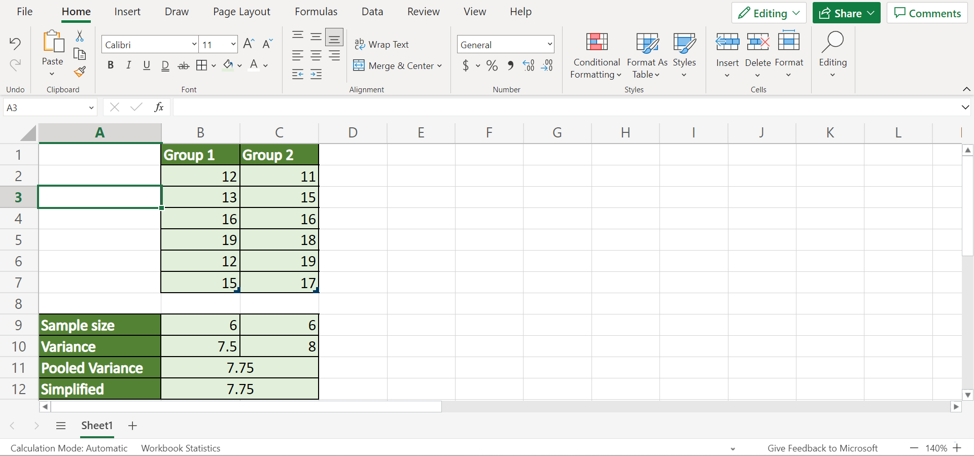
However, our two groups have the same sample sizes, so we can use the simplified formula version to calculate the pooled variance. And our final data set would look like this:
You can make your own copy of the spreadsheet above using the link attached below.
Amazing! Now we can learn the steps of how to calculate pooled variance in Excel.
How to Calculate Pooled Variance in Excel
In this section, we will discuss the step-by-step process of how to calculate pooled variance in Excel. Furthermore, each step contains detailed instructions and pictures to help you through the process.
To apply this method, simply follow the steps below.
1. Firstly, we need to individually convert the columns containing the two groups into tables. To do this, we will select the Group 1 column and go to the Insert tab. Then, we will select Table.

2. When the Create Table window appears, we will check My table has headers. Lastly, click OK to apply the changes.

3. Thirdly, we will go to the Table Design tab and uncheck the Filter Button and Banded Rows from the Table Style Options. Afterward, we will input the name “Group1” in the Properties section.
And we will repeat this process to the column containing Group 2.

4. Next, we will calculate the sample size using the COUNT function. So we will create a new row to input the results of the sample sizes. Then, we will type in the formula “=COUNT(Group1[Group 1])”. Lastly, we will press the Enter key to return the result.

5. Similarly, we will apply the same formula “=COUNT(Group2[Group 2])” for Group 2. Since they are two separate tables, we cannot use the Fill Handle tool to copy the formula.

6. Then, we will calculate the variance of each group using the VAR.S function. So we will create another row to input the result. Next, we will type in the formula “=VAR.S(Group1[Group 1])”. Finally, we will press the Enter key to return the result.

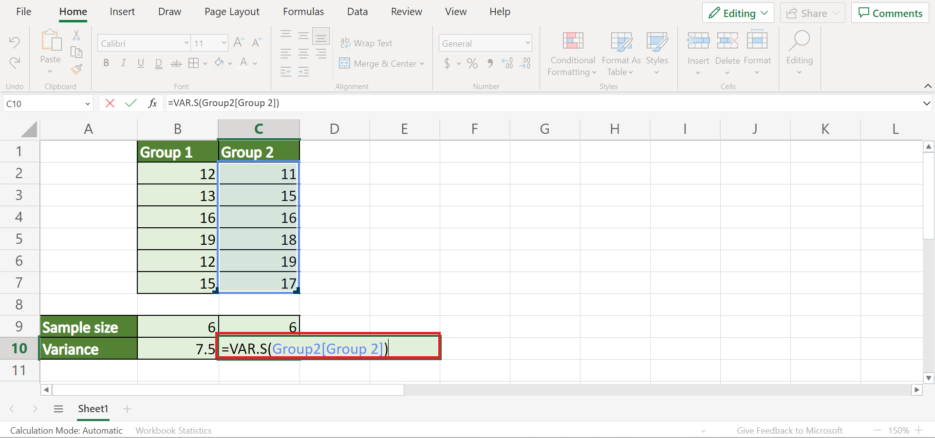
7. Again, we will apply the same formula to Group 2. So we will input the formula “=VAR.S(Group2[Group 2])”. Next, press the Enter key to return the result.
8. Lastly, we can calculate the pooled variance using the formula. So we will make a new row to input the result. Then, we will type in the formula “=((B9-1)*B10+(C9-1)*C10)/(B9+C9-2)”. Finally, press the Enter key to return the result.

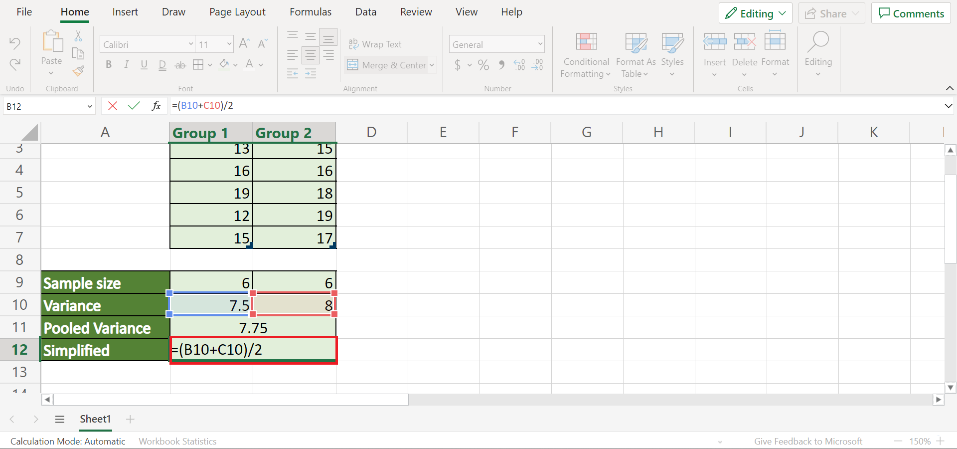
9. Alternatively, we can use the simplified formula since our sample sizes are the same. So we will input the formula “=(B10+C10)/2”. Lastly, we will press the Enter key to return the result.
10. And tada! We have successfully calculated pooled variance in Excel.
And that’s pretty much it! We have successfully explained how to calculate pooled variance in Excel using the VAR.S function. Now you can apply this method whenever you need to determine pooled variance among two or more groups.
Are you interested in learning more about what Excel can do? You can now use the VAR.S function and the various other Microsoft Excel formulas available to create great worksheets that work for you. Make sure to subscribe to our newsletter to be the first to know about the latest guides and tutorials from us.