This is the ultimate guide on how to combine ranges or arrays in Excel using two functions.
The rules for using the VSTACK function and the HSTACK function in Excel are the following:
- Both functions can combine ranges of cells, named ranges, array constant, and even dynamic arrays returned by other formulas.
- Because both functions return the results in an array that automatically spills into as many cells as needed, we only need to input the formula in one cell, which is the leftmost cell of the designated range.
- Both functions return a dynamic output. So any changes in the original arrays will automatically reflect or update in the returned array.
Excel has many useful tools and functions that make many tasks easier and more efficient. However, one of the things that used to be difficult to perform in Excel was combining two or more ranges together. But, not anymore!
Because Excel now has two functions we can utilize to combine ranges or arrays, this task has never been easier. Now we can merge ranges and arrays without difficulty, even dynamic ones.
And the functions we will be using to combine ranges or arrays in Excel are the VSTACK function and the HSTACK function. So the VSTACK function combines multiple ranges or arrays vertically into one array. While the HSTACK function is used to combine ranges or arrays horizontally into one array.
With the VSTACK function and the HSTACK functions, we can combine ranges or arrays in Excel vertically and horizontally depending on what fits best for our data set.
Let’s take a sample scenario wherein we need to combine ranges or arrays in Excel.
Suppose you are creating a product inventory. So you have three ranges for three different categories of products. For easier inventory checking, you want to combine all the ranges into one array.
Instead of manually typing each product, you opted to use the HSTACK function to make this task easier and more efficient. Now you have quickly finished combining the products into one inventory.
Great! Before we move on, let’s first learn how to write the VSTACK function in Excel.
The Anatomy of the VSTACK Function
The syntax or the way we write the VSTACK function is as follows:
=VSTACK(array1, [array2], ...)
Let’s take apart this formula and understand what each term means:
- = the equal sign is how to activate any function in Excel.
- VSTACK() is our
VSTACKfunction. And this function vertically stacks arrays into a single array. - array1 is a required argument. And this refers to the array or cell reference we want to stack vertically.
- array2 is an optional argument. And this refers to other arrays we want to vertically stack together.
Next, let’s learn how to write the HSTACK function in Excel.
The Anatomy of the HSTACK Function
The syntax or the way we write the HSTACK function is as follows:
=HSTACK(array1, [array2], ...)
Let’s take apart this formula and understand what each term means:
- = the equal sign is how to begin any function in Excel.
- HSTACK() refers to our
HSTACKfunction. And this function will stack the selected arrays horizontally. - array1 is a required argument. So this refers to the array we want to stack horizontally.
- array2 is an optional argument. And this refers to other arrays we want to stack together horizontally.
Amazing! Now let’s dive into a real example of combining ranges or arrays in Excel.
A Real Example of Combining Ranges or Arrays in Excel
Let’s say we have three sets of ranges containing different categories of products. And we want to create an inventory containing all the data coming from the three arrays. So our initial data set would look like this:

Instead of individually typing the products from all three ranges, we can utilize the VSTACK function and HSTACK function to combine the three ranges into a single one. And these are some straightforward functions.
So we simply need to select the arrays we want to combine. Then, we’re done! It is easy and simple to use the VSTACK function and HSTACK function.
Furthermore, we can include headers in the returned array of the functions. So we can simply select the headers together with the ranges so we can have headers in the return array of the function.
For example, the three ranges containing the products have a header or column name. Since we will be combining them together, we do not want to mix the different categories of products. But, worry not! We can include the headers directly in the VSTACK function or HSTACK function.
Additionally, we can also handle blank cells. For instance, the VSTACK and HSTACK functions will input the value 0 for blank or empty cells by default. But, we want to just leave those cells blank or empty for future inputting of data.
To do this, we can simply use the substitute function together with the VSTACK function or HSTACK function to replace the 0 with an empty space or character of the returned array.
After using the VSTACK function or HSTACK function to combine ranges or arrays in Excel, our final output would look like this:

You can make your own copy of the spreadsheet above using the link attached below.
Great! Finally, let’s dive into the process of how to combine ranges or arrays in Excel.
How to Combine Ranges or Arrays in Excel
In this section, we will discuss the step-by-step process of how to combine ranges or arrays in Excel using the VSTACK function and the HSTACK function. Furthermore, we will also discuss other actions we can perform using the two functions.
1. Firstly, let’s try combining the ranges vertically. So we will be utilizing the VSTACK function for this one. To do this, simply type the formula “=VSTACK(A2:A4,A7:A9,A12:A14)”. Then, press the Enter key to return the results.

2. And tada! We have successfully combined ranges or arrays in Excel vertically using the VSTACK function.

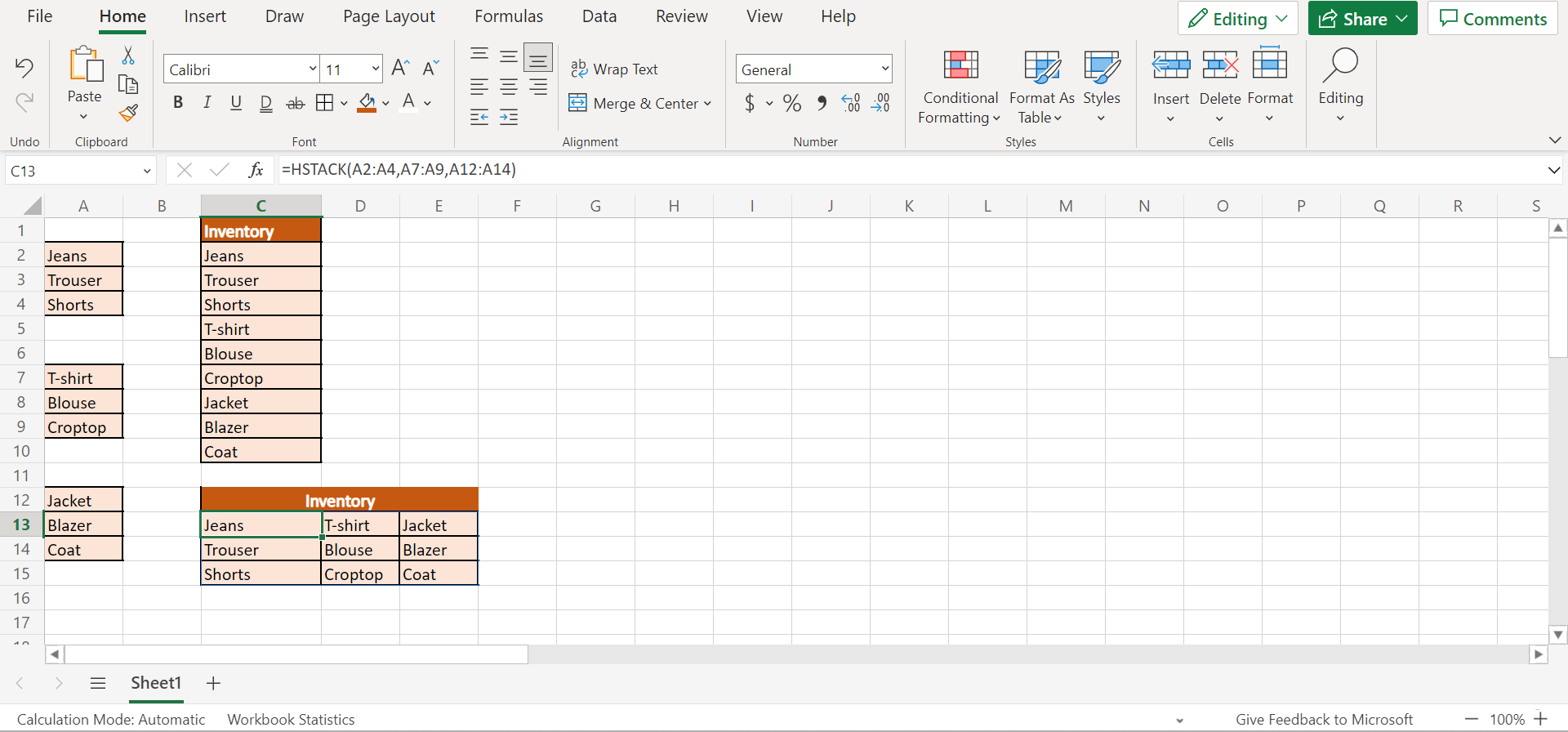
3. Secondly, let’s try combining the ranges horizontally. And this time, we will use the HSTACK function. So simple type in the formula “=HSTACK(A2:A4,A7:A9,A12:A14)”. Next, press the Enter key to get the results.

4. And tada! We have combined the ranges horizontally using the HSTACK function.
5. Thirdly, let’s try including headers in the returned array. For instance, we want to separate the ranges by category. In this case, we will have the headers, bottoms, tops, and outerwear.
To do this, type in the formula “=VSTACK(A1:A4,A6:A9,A11:A14)”. Lastly, press the Enter key to return the array with headers.
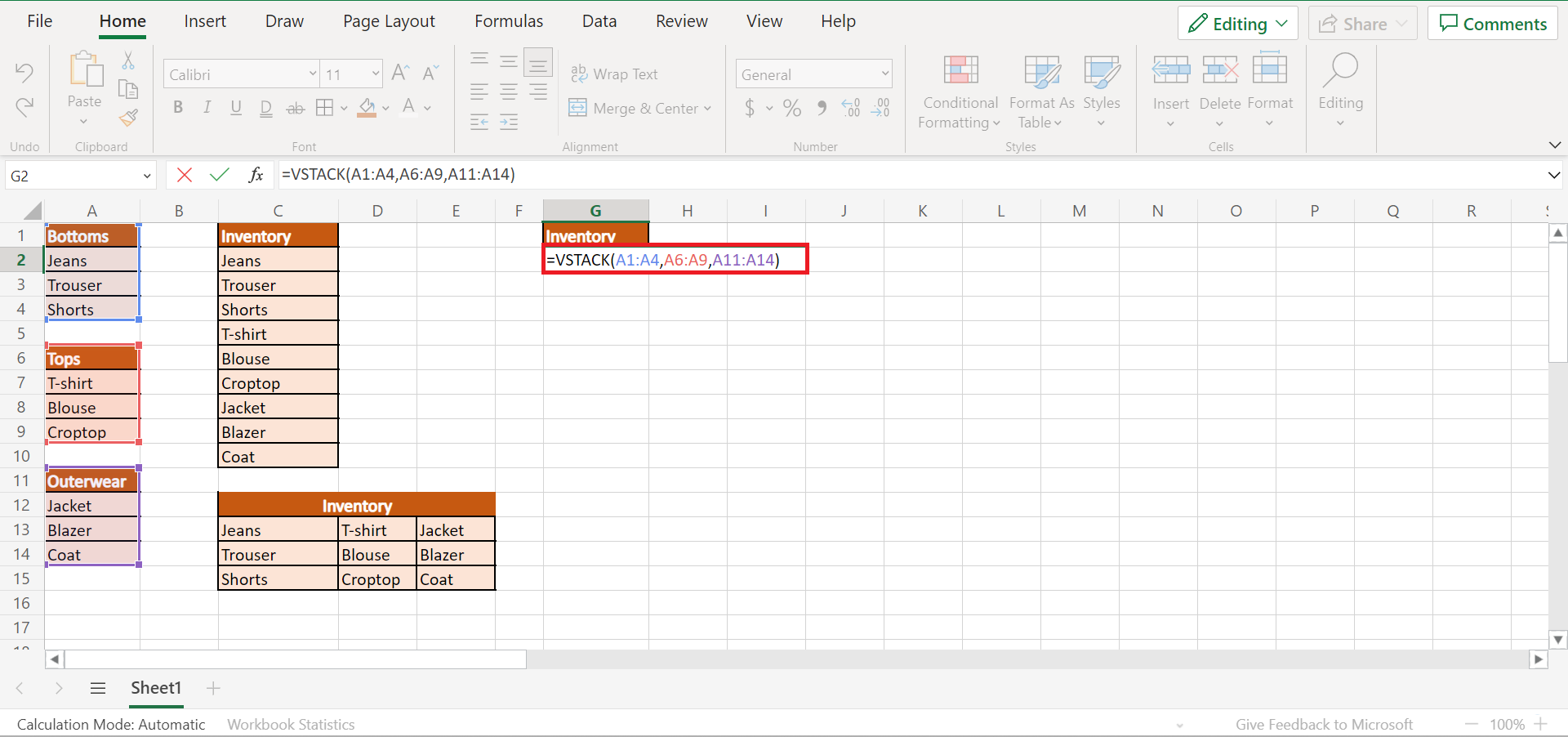
6. Great! Now we have included headers in the returned array.

7. Lastly, let’s replace 0 in the blank cells. To do this, we will use the substitute function together with the HSTACK function. So type in the formula “=SUBSTITUTE(HSTACK(A1:A14), 0, “”)”. Next, press the Enter key to return the array.
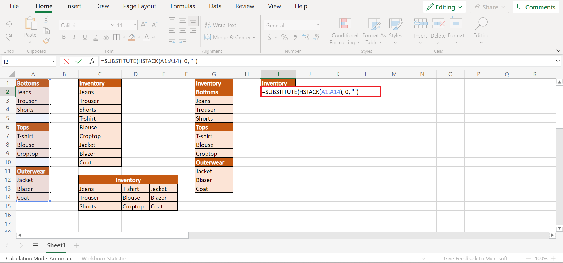
8. And tada! We have inputted a value in the empty or blank cells.
And that’s pretty much it! We have explained how to combine ranges or arrays in Excel using two functions. Now you can apply this whenever you need to combine ranges or arrays.
Are you interested in learning more about what Excel can do? You can now use the VSTACK function, the HSTACK function, and the various other Microsoft Excel formulas available to create great worksheets that work for you. Make sure to subscribe to our newsletter to be the first to know about the latest guides and tutorials from us.