How to Create Barcode In Google Sheets

The provision to create barcodes in Google Sheets is very useful and simple compared to the other functions and built-in capabilities. These could prove to be extremely important in domains such as retail, where product identity is easily tagged using a barcode.

That is all fine, but what is the real utility of a barcode? Barcodes save us from making manual errors – as simple as that. When you enter data yourself, it by design is more error prone, since a product tag usually consists of a combination of six to eight digits. A barcode scan saves you significant time compared to manually entering data. It is very simple to do as well, reducing the effort to learn the same. Could you ask for more, really?

Let’s take an example.

I plan to start a retail store in my vicinity and my planned product assortment ranges from hardlines to apparel. Manually entering and capturing sales data by product ID is going to be both cumbersome and error prone. For faster execution of transactions and ease of tracking sales volume, I would definitely need a technique that is both robust and scalable.

Here is where a barcode will come to my rescue. A barcode will ensure that the product tag is safely and, more importantly, uniquely captured.

Great! Let me take you through a real world use-case, and learn how we can write our own function in Google Sheets to create a barcode. There are two ways to creating barcodes in Google Sheets, and I shall take you through each of them, separately.

Anatomy of the Function: Method 1

So the syntax (the way we write) of the function is as follows:

=”*”&<cell_number>&”*”

Let’s dissect this thing and understand what each of the terms means:

• = the equal sign is just how we start any function in Google Sheets.
• “*” is just the ‘ampersand’ symbol wrapped in double quotes.
• <cell_number> denotes the reference to the cell which contains the product ID for which the barcode is to be created
• “*” again, is just the ‘ampersand’ symbol wrapped in double quotes.

A Real Example of using an ampersand and cell reference

Take a look at the example below to see how to create a barcode on Google Sheets:

The above are product listings at the neighborhood coffee shop, and you can clearly see that each coffee has a separate product ID. All of these are offered as takeaways, and therefore, the owner needs to tag the products with unique IDs for ease of transaction at checkout. This can easily be achieved using the aforementioned formula using an ampersand and cell reference, as shown below:

You may try changing it on your own with different product IDs, and see if you’re getting it right. Go ahead and make a copy of the spreadsheet using the link I have attached below:

But before you do, let me walk you through both the methods in detail on how to generate barcodes.

How to Create a Barcode in Google Sheets: Method 1

1. I have listed merchandise in the packaged food section at Starbucks in my neighborhood. The objective is to create barcodes for each of the product items so that they are unique.

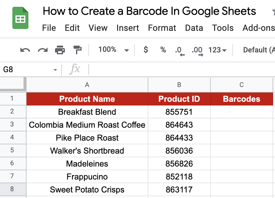
2. Now, simply click on any cell to make it the active cell. For this guide, I will be selecting C2, where I want to show my results.
3. Next, simply type the equal sign ‘=‘ to begin the function, followed by the asterisk symbol wrapped in double quotes, like this: “*”.
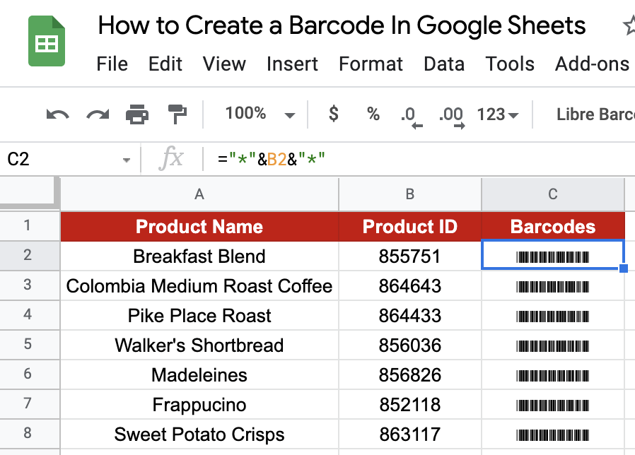
4. Continue by typing the ampersand symbol: ‘&’ and navigating to the cell which has the product ID listing, which in our case is B2. Finish the formula by typing the ampersand symbol again, followed by an asterisk symbol wrapped in double quotes. If you’ve typed it correctly, the final formula should look something like this:

5. Just hit your enter key now. You should see a number appear as the result. If Google Sheets suggests an Auto Fill (as shown below), go ahead and accept it, else drag the formula down all the way to cell B8 so that we have an output for each of the product IDs.

6. You’re nearly there. Select the barcode output (ini column C), and proceed to the Font name option. Select the ‘More Fonts’ option. 
7. Once you are on the Fonts tab, type in ‘Libre barcode’ in the search bar and select the first option, as shown below:

8. If you’ve followed all the steps correctly, you should have created barcodes for each of your product IDs as shown below. 

Awesome. Let us look at another way to create barcodes in Google Sheets.

Anatomy of the Function: Method 2

So the syntax (the way we write) of the function is as follows:

=IMAGE(url,[mode],[height],[width])

Let’s dissect this thing and understand what each of the terms means:

• = the equal sign is just how we start any function in Google Sheets.
• IMAGE() is the IMAGE function. IMAGE will return an image to the cell in which the formula is entered
• url – The URL of the image you want to insert into the cell
  • The url must either be enclosed in double quotes or a cell reference to the original link.
• mode – [ OPTIONAL – 1 by default ] – provides an option to resize the image
  • 1 fits the image to the cell, maintaining the original aspect ratio.
  • 2 fits the image to the cell, ignoring the aspect ratio.
  • 3 leaves the image at its original size, subject to potential cropping.
  • 4 allows the user to specify a custom size.
  • Note that no mode causes the cell to be resized to fit the image.
• height – [OPTIONAL] – denotes the height of the image in pixels; has a prerequisite of mode = 4.
• width – [OPTIONAL] – denotes the width of the image in pixels; has a prerequisite of mode = 4.

How to Create a Barcode in Google Sheets: Method 2

1. For ease of comparison and better understanding, we will be using the same data as in the previous example.

2. Now, simply click on any cell to make it the active cell. For this guide, I will be selecting C2, where I want to show my results.
3. Next, simply type the equal sign ‘=‘ to begin the function and then followed by the name of the function, which is our ‘image‘ (or IMAGE, whichever works).
4. You should find that the auto-suggest box appears with our function of interest. Continue by entering the first opening bracket ‘(‘. If you get a huge box with text in it, simply hit the arrow in the top-right hand corner of the box to minimize it. You should now see it as follows:

5. The first input to the function is the url. For this, go to the link: https://www.barcodesinc.com/generator/ and click on the ‘Make a Barcode Online – FREE’ option. On the landing page, enter the product ID for which you want to create the barcode for (855751 in this case) and click on “Generate Barcode”. You should see the windows as shown below:

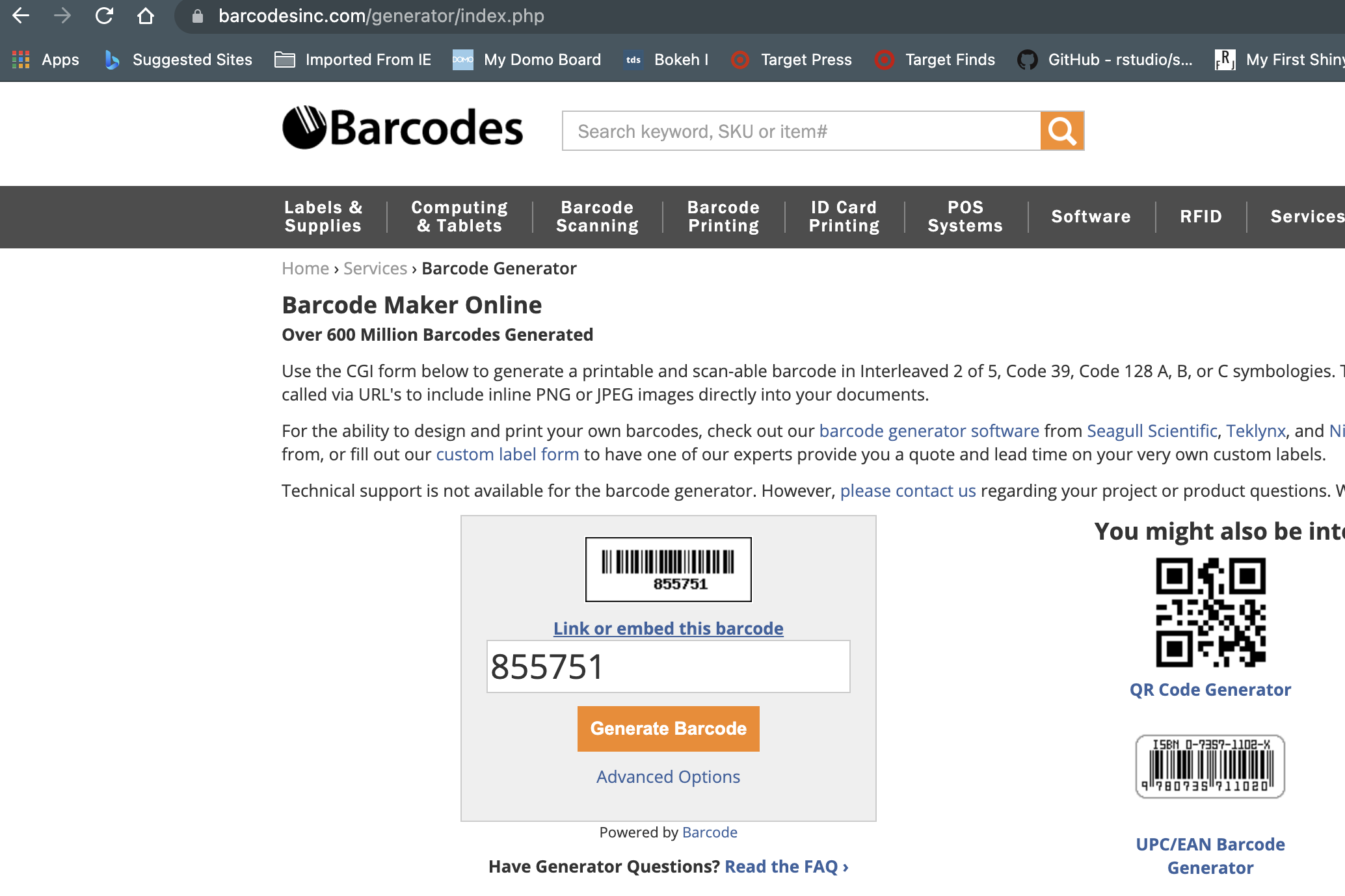
6. Proceed to click on the “Link or embed this barcode” option. You will see a link generated just below the option, and you have to copy the link. Then, go back to the Google Sheets tab and paste this link within quotes inside the IMAGE function as shown below:

8. Finally, replace the product ID 855751 within the link with this dynamic reference: “&C2&” and drag the formula down. If you followed all the steps correctly, you would have got the correct barcode created as shown below. 

That’s pretty much it. You have everything you need to get started with creating a barcode on Google Sheets. I recommend trying your hand at it, combining it with the numerous Google Sheets formulas available, and seeing what you can come up with. 🙂 Get cracking! 

Get emails from us about Google Sheets.

Our goal this year is to create lots of rich, bite-sized tutorials for Google Sheets users like you. If you liked this one, you'll love what we are working on! Readers receive ✨ early access ✨ to new content.

Subscribe