This guide will explain how to use the DURATION function in Google Sheets.
When we need to calculate the number of compounding periods required for an investment of a specified present value appreciating at a given rate to reach a target value, we can easily do this using the DURATION function in Google Sheets.
Table of Contents
The rules for using the DURATION function in Google Sheets are the following:
- The settlement and maturity arguments must be entered using the DATE, TO_DATE, or other date parsing functions rather than by entering text.
- If we omit the day_count_convention argument, the default value is 0, the US (NASD) 30/360-day count convention.
- The price and redemption values must be expressed as a percentage of the face value.
- We must make sure to enter dates in the correct format YYYY-MM-DD.
- The Macaulay duration is different from the modified duration, which is the
MDURATIONfunction, in that it measures the weighted average time for an investment to reach maturity.
Google Sheets offers several functions we can utilize to calculate different financial factors.
One of these functions is the DURATION function which is used to calculate the number of compounding periods required for an investment of a specified present value appreciating at a given rate to reach a target value.
Other examples are the YIELD function, the PRICE function, and the MDURATION function.
The DURATION function is beneficial in evaluating the number of compounding periods required before an investment reaches a target value. Moreover, we consider the settlement date, maturity date, rate, yield, frequency, and day count convention.
In this guide, we will provide a step-by-step tutorial on how to use the DURATION function in Google Sheets. Additionally, we will explore the syntax and a real example of using the function.
Great! Let’s dive right in.
The Anatomy of the DURATION Function
The syntax or the way we write the DURATION function is as follows:
=DURATION(settlement,maturity,rate,yield,frequency,[day_count_convention])
- = the equal sign is how we begin any function in Google Sheets.
- DURATION() refers to our
DURATIONfunction. This function is used to calculate the number of compounding periods required for an investment of a specified present value appreciating at a given rate to reach a target value. - settlement is a required argument. It refers to the settlement date of the security, the date after issuance when the security is delivered to the buyer.
- maturity is also a required argument. This is the maturity or end date of the security when it can be redeemed at the face or par value.
- rate is a required argument. This refers to the annualized rate of interest.
- yield is another required argument. It refers to the expected annual yield of the security.
- frequency is also a required argument. This refers to the number of interest or coupon payments per year.
- day_count_convention is an optional argument. It is an indicator of what day count method to use. By default, the value is 0, which indicates the US (NASD) 30/360 day count convention.
The Optional Argument of the DURATION Function
The DURATION function has several required arguments to work properly. However, there is only one optional argument that we can utilize to apply the appropriate day count method to get accurate results.
The day_count_convention is the only optional argument of the DURATION function, which allows us to indicate what day-count method to use in the formula.
By default, the value of the day_count_convention is 0 meaning the formula will use the US (NASD) 30/360-day count convention. This assumes there are 30 days in a month and 360 days in a year as per the National Association of Securities Dealers standard.
The value 1 indicates Actual/Actual, which is calculated based on the actual number of days between the specified dates and the actual number of days in the intervening years. This is often used for US Treasury Bonds and Bills, but also the most relevant for non-financial use.
If we input 2, we are indicating the Actual/360-day count convention. This is calculated based on the actual number of dates between the specified dates but assumes there are 360 days in a year.
The value 3 indicates the Actual/365-day count convention, which is calculated based on the actual number of days between the specified dates but assumes there are 365 days in a year.
Lastly, the value 4 indicates European 30/360. This is similar to the default 0, which is calculated based on the assumption that there are 30 days in a month and 360 days in a year. However, according to the European financial conventions, this day count convention will adjust the end-of-month dates.
We can refer to the table below for an easier overview of the day_count_convention argument.
| Value | Indicates | Description |
| 0 | US (NASD) 30/360 | 30-day months and 360-day year |
| 1 | Actual/Actual | Actual number of days and the actual number of days in the intervening years |
| 2 | Actual/360 | Actual number of days and 360-day year |
| 3 | Actual/365 | Actual number of days and 365-day year |
| 4 | European 30/360 | 30-day months and 360-day year, but adjusts end-of-month dates to European financial conventions |
A Real Example of Using DURATION Function in Google Sheets
Let’s say we want to calculate the number of compounding periods required for our investment to reach a target value with the following data:
- a settlement date of January 1, 2023
- a maturity date of January 1, 2030
- annual coupon payments
- an annual interest rate of 5%
- an annual yield of 10% using the Actual/actual day count convention
Our initial data set would look like this:
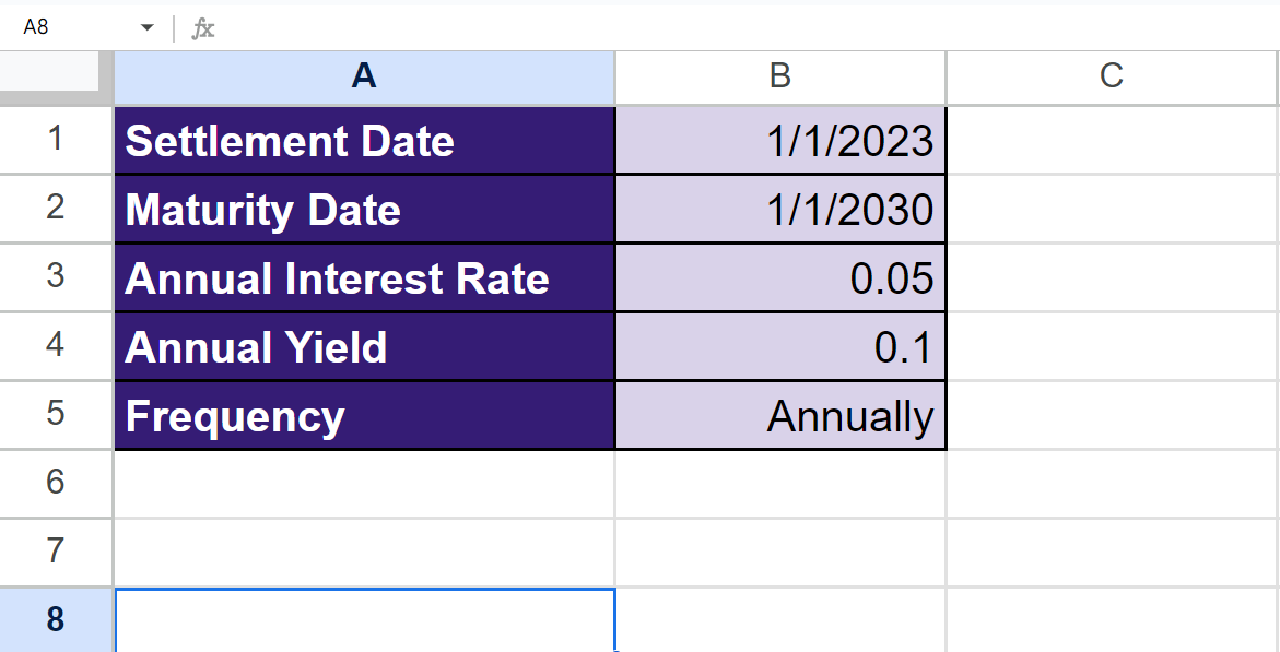
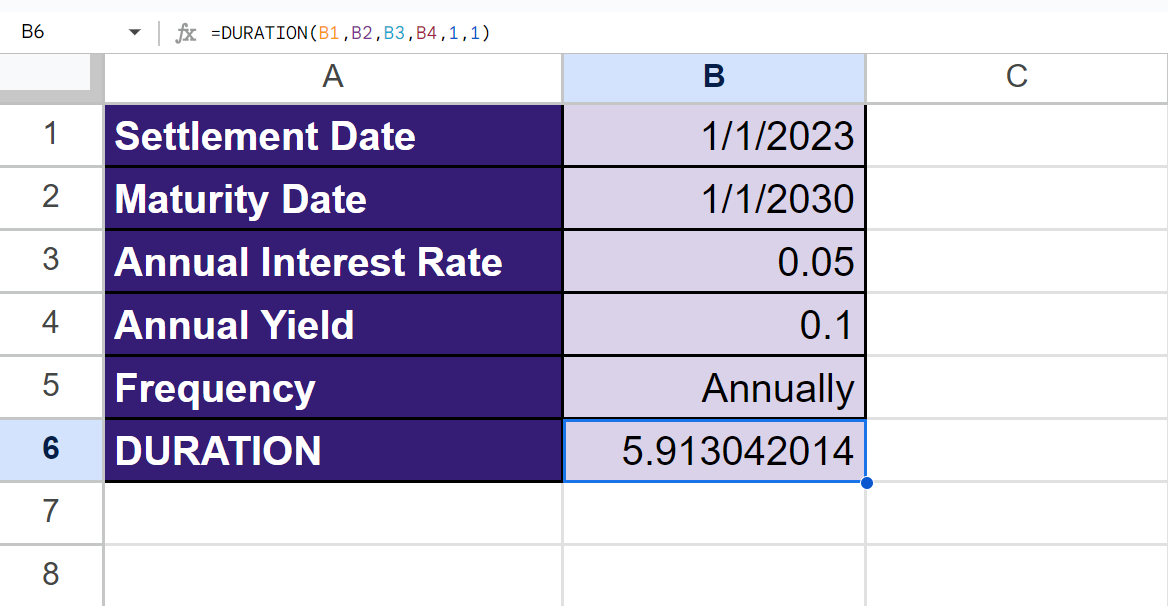
The spreadsheet above shows all the values we need to calculate the compounding periods. Additionally, we have the settlement date, the maturity date, the interest rate, the annual yield, and the frequency of coupon payments.
We can easily do this using the DURATION formula below:
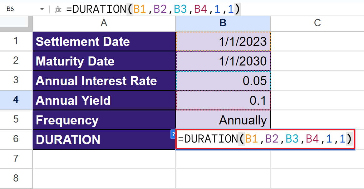
=DURATION(B1,B2,B3,B4,1,1)

In the formula above, we first selected the cell containing the settlement date, which is B1 (1/1/2023). Then, we selected the cell containing the maturity date, which is B2 (1/1/2030). Next, we simply selected the cell containing the annual interest rate, which is B3 (0.05).
Afterward, we also selected the cell containing the expected annual yield, which is B4 (0.10). Then, we typed in the 1 as our frequency since the coupon payment is annual. Lastly, we placed 1 as our day_count_convention to calculate based on the actual/actual day count.
Our final data set would look like this:

You can make your own copy of the spreadsheet above using the link below.
Amazing! Now we can dive into the steps of using the DURATION function in Google Sheets.
How to Use DURATION Function in Google Sheets
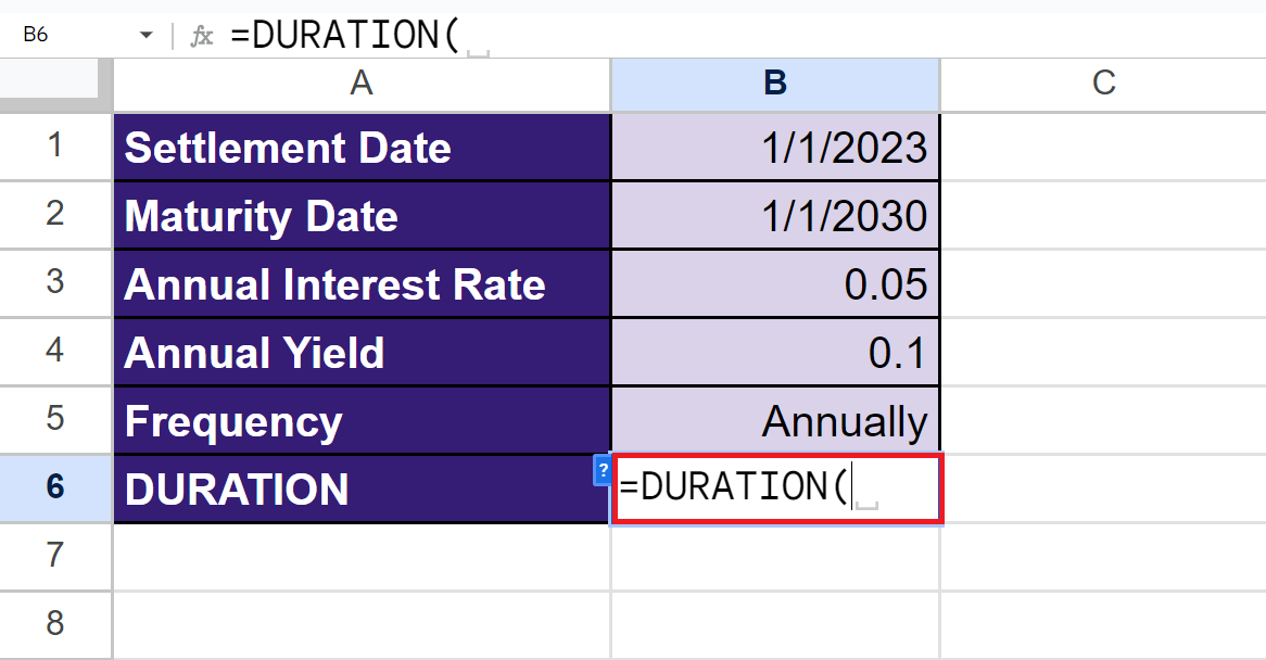
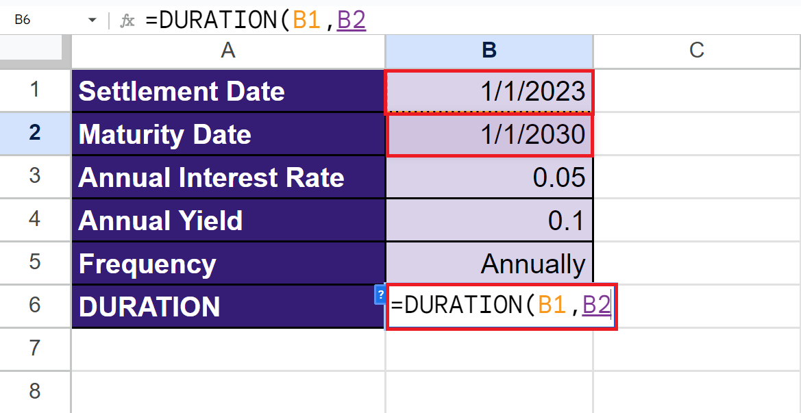
1. First, we will select an empty cell to type in our formula. To start, we will type in an equal sign and the function name. Our formula would start with “=DURATION(”.
2. Then, we will simply select the cells containing the settlement date and the maturity date. Our formula would become “=DURATION(B1,B2”.
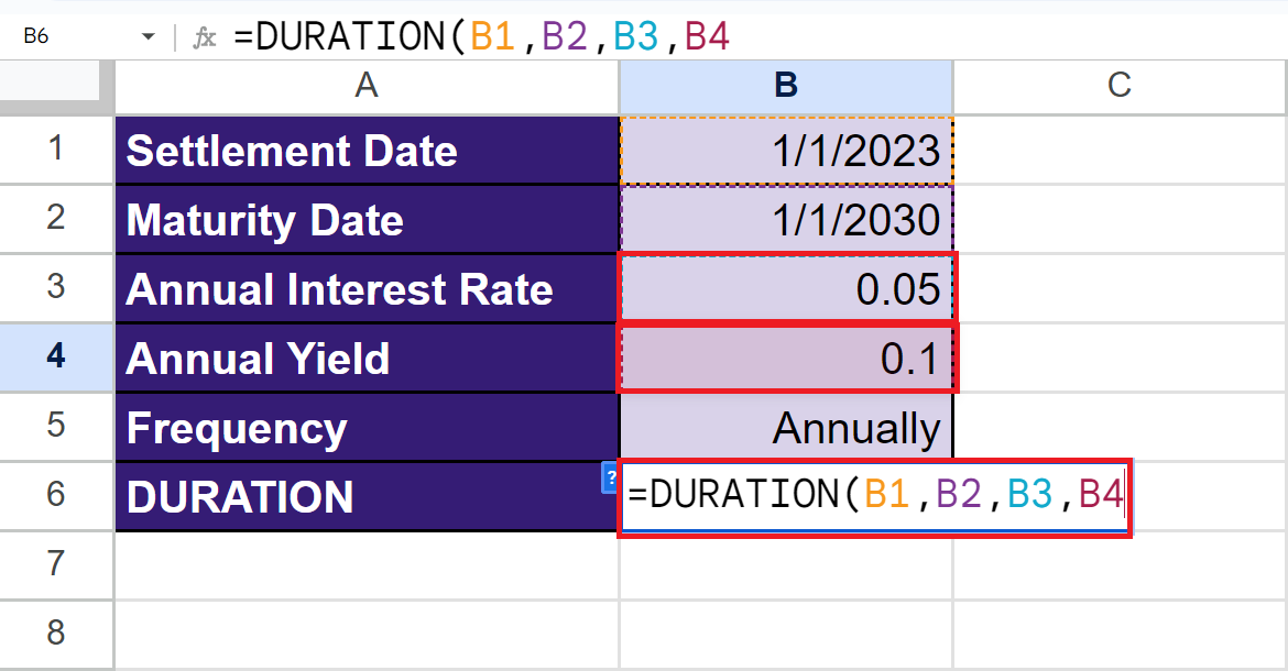
3. Next, we will select the cells containing the interest rate and the annual yield. Our formula would become “=DURATION(B1,B2,B3,B4”.
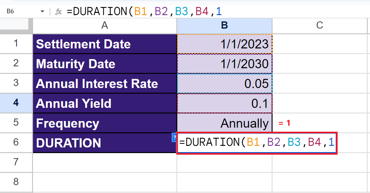
4. Afterward, we typed in the frequency of coupon payments. Our formula would become “=DURATION(B1,B2,B3,B4,1”.
5. Lastly, we will choose a day count method to use. In this case, we will input “1” to calculate based on the actual number of days in the dates and intervening dates. Our final formula would be “=DURATION(B1,B2,B3,B4,1,1)”.
6. We will press the Enter key to return the result.
And tada! We have successfully used the DURATION function in Google Sheets.
You can apply this guide whenever you need to calculate the number of compounding periods required for an investment to reach a target value. You can now use the DURATION function and the various other Google Sheets formulas available to create great worksheets that work for you.
That’s pretty much it! Make sure to subscribe to our newsletter to be the first to know about the latest guides and tutorials from us.