This guide will discuss how to use the EFFECT function in Google Sheets.
Table of Contents
When we need to calculate the annual effective interest rate given the nominal rate and the number of compounding periods per year, we can easily do this using the EFFECT function in Google Sheets.
The rules for using the EFFECT function in Google Sheets are the following:
- The nominal_rate must be in decimal format. For example, a 5% nominal rate will be inputted as 0.05.
- We will always use the effective annual interest rate when comparing loans and investments.
- The nominal_rate and perioeds_per_year must be positive values.
One of the many Google Sheets functions that let us calculate the effective annual interest rate is the EFFECT function.
The EFFECT function calculates the effective annual interest rate, considering the nominal annual interest rate and the number of compounding periods per year. This is particularly useful when comparing different investment options or loans with varying compounding periods.
In this guide, we will provide a step-by-step tutorial on how to use the EFFECT function in Google Sheets. Additionally, we will explore the syntax and a real example of using the function.
Great! Let’s dive right in.
The Anatomy of the EFFECT Function
The syntax or the way we write the EFFECT function is as follows:
=EFFECT(nominal_rate,periods_per_year)
- = the equal sign is how we activate any function in Google Sheets.
- EFFECT() refers to our
EFFECTfunction. This function is used to calculate the annual effective interest rate given the nominal rate and number of compounding periods per year. - nominal_rate is a required argument. It refers to the nominal interest rate per year.
- periods_per_year is also a required argument. This refers to the number of compounding periods per year.
Note: We can utilize the NOMINAL function when we want to calculate the nominal annual interest rate.
Common Mistakes in Using EFFECT Function
The EFFECT function has a straightforward syntax making it simple to use. However, we still need to be careful when using some things to ensure the function properly works.
Firstly, we may have entered a percentage value for the nominal_rate instead of a decimal value. Remember to divide the percentage by 100 to convert it to a decimal. The nominal_rate must always be inputted as a decimal.
Secondly, we may have placed a negative value on the nominal annual interest rate or the number of compounding periods per year. The nominal_rate and the periods_per_year arguments must always be positive values.
Thirdly, ensure that we have included both required arguments in the formula. If we miss one required argument, the function will return an error.
Lastly, check the syntax of the formula. Ensure the syntax of the function call is correct, including the proper placement of commas and the use of parentheses.
A Real Example of Using EFFECT Function in Google Sheets
Let’s say we have a loan with a nominal annual interest rate of 10% compounded monthly. We want to calculate the effective annual interest rate. Our initial data set would look like this:
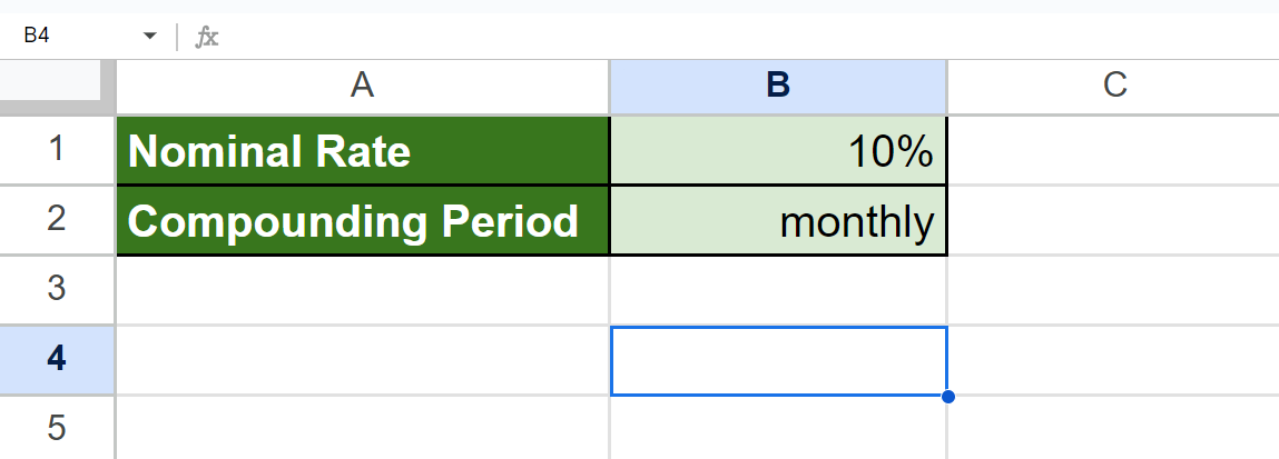
In the spreadsheet above, we can see the nominal interest rate per year and the number of compounding periods per year.
We can calculate the effective annual interest rate using the formula below:
=EFFECT(0.10,12)
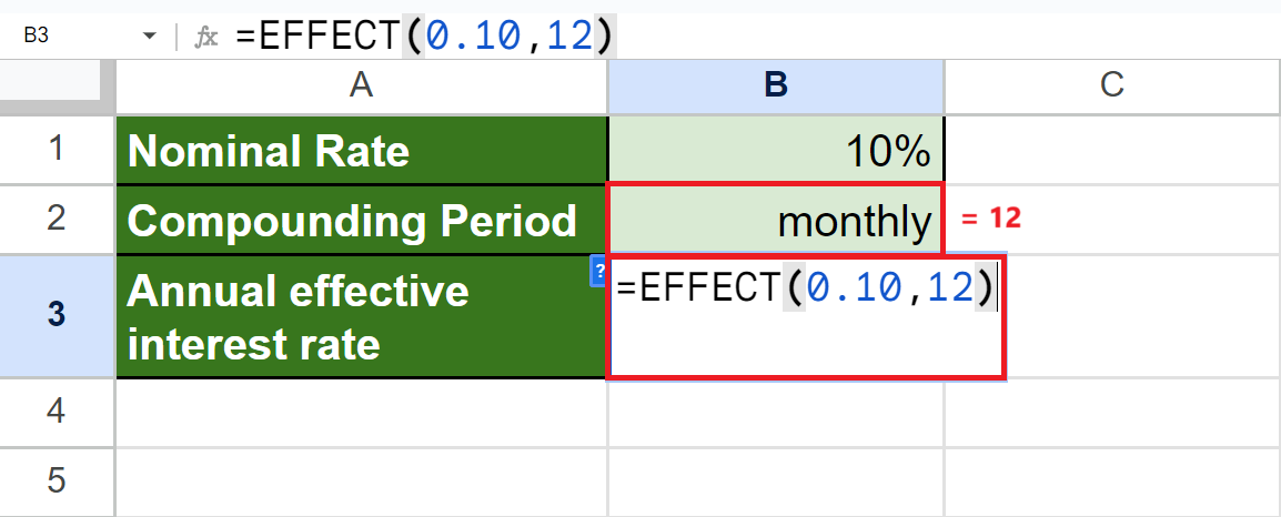
The first part of the formula is our nominal_rate. Since the nominal_rate is 10%, we typed in 0.10 in decimal format. Next, we inputted 12 as our periods_per_year value since the loan compounds monthly.
Our final data set would look like this:

You can make your own copy of the spreadsheet above using the link below.
Amazing! Now, we can dive into the steps of using the EFFECT function in Google Sheets.
How to Use EFFECT Function in Google Sheets
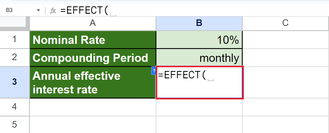
1. First, we will select an empty cell to type in our formula. To start, we will type in an equal sign and the function name. Our formula would be “=EFFECT(”.
2. Then, we will type in our nominal_rate in decimal format. Since our nominal_rate is 10%, our formula would be “=EFFECT(0.10”.

3. Next, we will input our periods_per_year value. Since the loan compounds monthly, the value would be “12”. Our final formula would be “=EFFECT(0.10,12)”.

4. We will press the Enter key to return the result.

And tada! We have successfully used the EFFECT function in Google Sheets.
You can apply this guide whenever you need to calculate the annual effective interest rate given the nominal rate and number of compounding periods per year. You can now use the EFFECT function and the various other Google Sheets formulas available to create great worksheets that work for you.
FAQs:
1. I already have the effective annual interest rate value. How do I find the nominal annual interest rate?
You can use the NOMINAL function, which calculates the annual nominal interest rate given the effective rate and number of compounding periods per year.
2. How do I compare loans with different compounding periods?
To compare loans with different compounding periods, you would have to calculate the effective annual interest rate of each loan.
For example, there are two loans with the same nominal annual interest rate but different compounding periods per year. You can simply use the EFFECT function and input the different compounding periods.
EFFECT=(O.O5,4) // loan compounded quarterly
EFFECT =(0.05,12) // loan compounded monthly
3. What are other related functions?
The INTRATE function calculates the effective interest rate generated when an investment is purchased at one price and sold at another with no interest or dividends generated by the investment itself.
Other related functions are the FV function, the PV function, and the IPMT function.
That’s pretty much it! Make sure to subscribe to our newsletter to be the first to know about the latest guides and tutorials from us.