How to Find the Last Matching Value in Google Sheets

To find the last matching value in Google Sheets is useful if you want to find the last occurrence of a specified value in a list.

You might want to learn how to do it if you are using a constantly changing, dynamic sheet that you update regularly, and you need information about the latest occurrence of something.

Let’s take an example.

Say you deliver a daily lunch menu, and you want to create a sheet where you save the type of food you served each day. 🥪🍕

You want to search for food types and see easily when was the last time you served that food.

So how do we do that?

It’s easy. We need to find the last matching value in the list.

The combination of the LOOKUP and the SORT functions help us do that. It searches through a sorted row or column for a key value and then returns the value of the cell. The value of the cell is in a result range located in the same position as the search row or column.

Now don’t worry if you do not understand what anything means. By the end of this post, you will have gained a greater understanding of all this, so bear with us. 😅 But first, let’s talk about the LOOKUP function to understand how it works before we move any further.

The Anatomy of the LOOKUP Function

The syntax (the way we write) the LOOKUP function is as follows:

=LOOKUP(search_key, search_range, result_range)

Let’s break this down so we can get a better understanding of what each of those terms mean:

• = the equal sign is how we start just about any function in Google Sheets.
• LOOKUP is our function. We will have to provide it with the search_key, search_range and result_range to make it work.
• search_key is the value that we want to search for in the selected row or column.
• search_range is the range of cells where we search for the search_key.
• result_range will be the range of cells, from which the formula returns a result. The value returned corresponds to the location where search_key is found in search_range.

⚠️ Note About the Syntax of LOOKUP

Be aware that this is not the only way to write the LOOKUP function and exists another syntax of this function.

The other one is used for cases when you want to get the result from the same range than your search range. But for our example now, we use this above version to find the last matching value.

A Real Example of Using LOOKUP Function

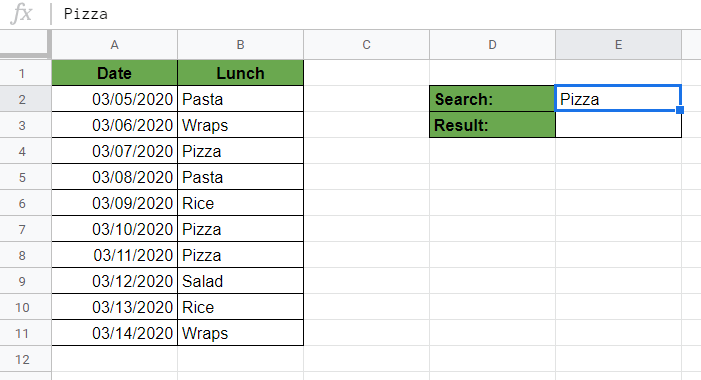
Have a look at the example below to see how to use LOOKUP to find the last matching value in the list. Let’s see the sheet of our food delivery service.

The above image shows how to use the LOOKUP function together with the SORT function to find the date where a type of food was last served. The function is as follows:

=LOOKUP(E2, SORT(B2:B11), SORT(A2:A11,B2:B11,TRUE))

Now, why do we need the SORT function?

The reason is that the LOOKUP function only works with sorted data.

So we need to sort our ranges to be able to use them in LOOKUP. Furthermore, it is crucial that we sort our ranges in the same order. The SORT function is the way to do this.  If you would like to read the details on how to use SORT function in Google Sheets, check out our guide.

Here’s what this example does:

• We wrote our LOOKUP function with the three variables separated by commas.
• We have written “Pizza”, the term we want to look up, in the cell E2. This can be any food from the list.
• The first variable we need to write in the LOOKUP formula is the search_key, so this is the term we want to lookup in the column. We used a cell reference here, so we wrote E2 because this cell has our search key.
• The second variable of the LOOKUP function is the search_range. Therefore, we put the range of B2:B11 here, because this range is where we want to search for the search_key.
• We also had to sort the range in ascending order (the default search order of SORT) to make it work with the LOOKUP function, so the second variable is: SORT(B2:B11).
• The third variable of the LOOKUP function is the result_range, so the range where we want to get our result from. We must sort the result_range according to the search_range, so we had to write a SORT formula here as well.
• The range we sort is the column containing the dates (SORT). The range by which to sort the data is the column with the food names (B2:B11). Finally, we define the ascending order by adding TRUE at the end. The whole result_range looks like this: SORT(A2:A11, B2:B11, TRUE).
• In summary, we added these three variables into the LOOKUP function, and after writing the whole formula in cell E3, we got our result: “3/11/2020” which is the date where we last had pizza in the list.
• We can now change the search term to any other food from the list, and the formula will automatically give us the last matching date.

See how easy it is?

Make a copy of the spreadsheet from the link I’ve attached below and try it for yourself:

How to Find the Last Value in Each Row in Google Sheets

Here you can see the step-by-step process on how to find the last matching value in Google Sheets with the LOOKUP function combined with SORT.

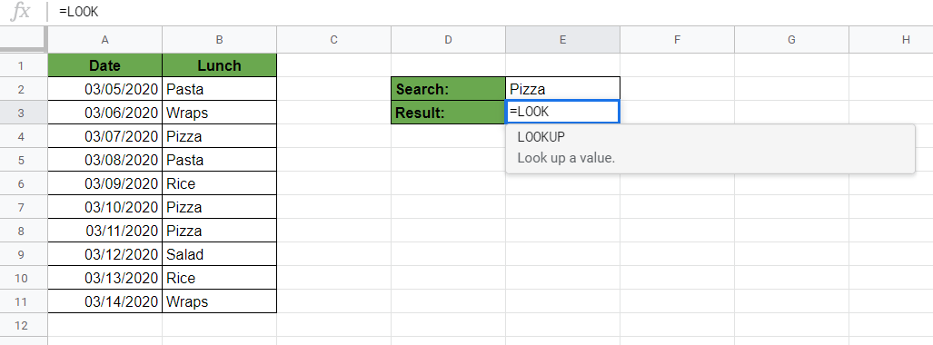
1. To start, write the search term that you want to look up in any cell. For this guide, I write “Pizza” in cell E2.

2. Next, select any cell where you want to show your result of the search. This is the cell where you will write your LOOKUP formula. For example, choose the cell E3 by clicking on it.

3. Enter the equal sign ‘=’ to begin the function. Then followed by the name of the function which is ‘lookup‘ (or ‘LOOKUP‘, whichever works).

4. Great job! You should now see the pop-up auto-suggest box with the name of the function LOOKUP.

5. After having entered the opening bracket ‘(‘, you will have to add the corresponding variables for the function to work. Firstly, add the first variable, which is the key value we are looking for. Click on the cell that has the search_key. That is, the cell E2 for me.

6. After that, you need to add the search_range variable which should be the sorted list of the food names. Start by writing the name of the SORT function and select it from the auto-suggest box. Make sure to choose the right function, because there are more functions with similar names.

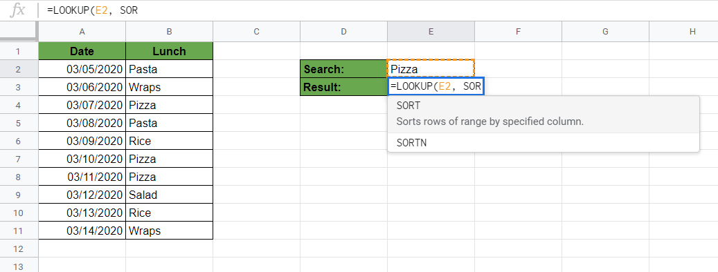
7. Now, put the range of cells in the SORT function where your food names are located. In my example, this is the range B2:B11, but since the list might be expanded later, I will include the whole column B starting from B2 and below. So the range I write here is B2:B.

8. After closing the brackets on this SORT function, put a comma to separate it from the third variable of the LOOKUP formula.

9. Now, write your third variable which is the result_range. This should also be a sorted list containing the dates (the possible results we might get). So write another SORT formula.

10. Put the range that has the possible results, so the range of the dates into it first. In the same way as before, this is A2:A for me because I want to include the whole column A where the future values will be added.

11. Afterwards, highlight the range of cells by which you want to sort the dates (the range of the food names, B2:B in my sheet).

12. Finally, set the ascending order of this sorting by writing TRUE at the end of the formula.

13. To finish, hit the Enter key to close the brackets and get the result of the formula. That’s it! You can see the last matching value in cell E3.

That’s pretty much it! You can now use the LOOKUP and SORT functions to find the last matching value in Google Sheets. You can even pair what’ve you learnt together with the other numerous Google Sheets formulas to create even more powerful formulas. 🙂

Get emails from us about Google Sheets.

Our goal this year is to create lots of rich, bite-sized tutorials for Google Sheets users like you. If you liked this one, you'll love what we are working on! Readers receive ✨ early access ✨ to new content. There will be no spam and you can unsubscribe at any time.

Subscribe