How To Highlight Cells Containing Specific Function In Google Sheet

Have you ever wondered how to highlight cells containing specific function in Google Sheets to make them stand out from the rest of the cells?

You might have come across a Google Sheet where some columns are formatted differently than others. In fact, this type of formatting is necessary to highlight columns or rows that might be relatively more important for the intended audience. 

Therefore, in this article, we hope to teach you how to highlight cells with specific functions. We also aim to make this guide as simple as possible by adopting a divide-and-conquer approach. First, we will look at the two essential functions FORMULATEXT and REGEXMATCH. Then, we will see how these functions work together to highlight cells containing specific functions in Google Sheets.

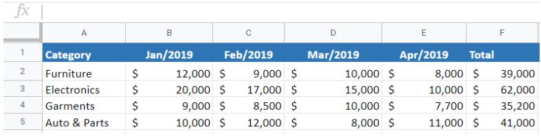
We will be using our very own sales record Google Sheet throughout this tutorial. To get familiar with it, have a look at the image. You can see the sales of different products from January 2019 to March 2019.

So how do we go about this?

To get a clear idea you need to learn about the two essential functions first and then move to the tutorial. At the end of the tutorial, we expect you will be able to perform the same steps for every function of your choice.

The Anatomy of FORMULATEXT Function in Google Sheets

The syntax (the way we write) of the FORMULATEXT function is as follows:

=FORMULATEXT(cell)

Let’s have a look at each part of the function to understand what is going on here:

• = is the equal sign that starts off any function in Google Sheets.
• FORMULATEXT is the name of our function.
• cell refers to a single or a range of cells.

Note that if a range of cells is passed in FORMULATEXT, only the top leftmost cell is evaluated.

An Example of Using FORMULATEXT Function

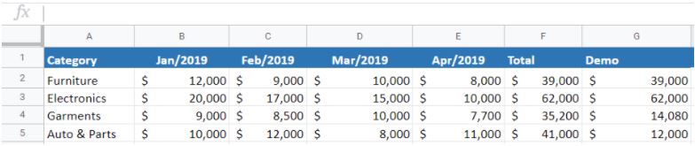
We have seen the sales record Google Sheet above. A column “Demo” has been added to it. The value in each of its cells is an output of a formula. We need to view what formula has been used at each cell in column G. Therefore, we will use the FORMULATEXT function.

To begin with it, we need another column at H. We will name it “Formula Text“. In the cell H2, we will enter the formula. The formula looks like this:

=FORMULATEXT(G2) 

Once we enter the formula and press ENTER, it will then show us the actual formula present in the cell G2.

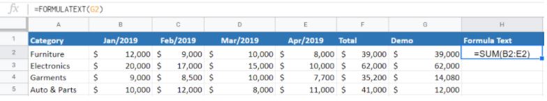
We can also see a blue square icon in the bottom right of cell H2. We will right-click on it and drag it down to H5. This will then copy FORMULATEXT for the rest of the cells. Now, can you guess the output? Let’s see the output.

We can observe what happens after we apply FORMULATEXT(cell) to column H with corresponding cells from G as the cell parameter. It returns the actual formula as text. Quite straightforward, isn’t it?

This simple problem can be practiced to perfection. Use the link below to get a copy of this problem set:

I assume the FORMULATEXT function is easier to understand. We now move on to our next function, REGEXMATCH.

The Anatomy of REGEXMATCH Function in Google Sheets

Before we dive into specifics of the REGEXMATCH function, we will try to know what regex is.

Regex

Regex stands for Regular Expression. It is a sequence of characters that defines a string pattern. Different algorithms use regex to find and match a string based on it. Beginners can go through the Regex tutorial to learn more. Google products use RE2 for regular expressions.

The syntax of the REGEXMATCH function is as follows:

=REGEXMATCH(text,regular_expression)

• = is the equal sign that starts off any function in Google Sheets.
• REGEXMATCH is the name of our function.
• textis the parameter that needs to be matched by the algorithm against a regular expression. 
• regular_expression defines a pattern.

An Example of Using REGEXMATCH Function

Let’s continue with our sales record sheet. We will add a “Random Text” column to it. This column contains some random text.

We will then try to match the text in the Random Text against a regular expression. This example includes regular expressions from the table.

Based on the regular expression in the table, we will try to match strings in column G. We would add column H to show exactly which regular expression are we using. The equation, therefore, takes cell references from column G. In the case of G1 the formula becomes:

=REGEXMATCH(G1,"[A-Za-z]+")

We then put this formula in cell I1.

We will then repeat this formula for cells I2 to I5 and replace the parameters accordingly for each cell. The final output is shown as:

We can see that entries in the Random Text column match against their corresponding Regular Expression in the Regular Expression column. Therefore, we get TRUE in every cell of the output column.

This simple problem can be practiced to perfection. Use the link below to get a copy of this problem set:

How to Highlight Cells Containing Specific Functions in Google Sheets: Step-by-Step

1. 1. Let’s start with a new sheet. We will enter some numbers in the first row from range A1:D1.

1. 2. In column E we will activate cell E1 by clicking on it, we will insert the SUM function by typing “=SUM(A1:D1)”, either in the cell itself or the formula bar above.

1. 3. Press the Enter key and you should then get your entries from A1 to D1 summed up in cell E1.

1. 4. Now, cell E1 is the only cell that contains a formula. We aim to highlight it. We will use what is called Conditional formatting. To access it, we then need to click on the Format drop-down in the top-most menu and navigate to Conditional Formatting.

1. 5. Now, click on Conditional Formatting. A menu then appears on the right side.

1. 6. In the Conditional Formatting menu, click on the square grid icon under the Apply to range. This will then open up a box with an option to select a data range.

1. 7. Select a data range would prompt us to select the region of our interest. Let’s select the entire first row by right-clicking and dragging the mouse across it. After selecting the range, click on OK.

1. 8. After selecting a data range, we will then move back to the conditional formatting menu to select Custom formula is under the Formula rules.

1. 9. In the custom formula, we then type our custom formula. The custom formula is:

=REGEXMATCH(FORMULATEXT(A1),"(?i)FUNCTIONAME")

1. 10. We will search for cells with the SUM function. Let’s plug-in SUM in the custom formula. It therefore becomes:

=REGEXMATCH(FORMULATEXT(A1),"(?i)SUM")

1. 11. Click on Done and you are good to go. Furthermore, you can change the style using the Formatting style in the conditions formatting menu. Voila!

Finally, We have seen how to highlight cells containing specific function in Google Sheets.

We can iterate these steps for any function, with a slight modification to the custom formula. All you need is to replace the FUNCTIONAME in the custom formula with a function of your choice.

For your ease, we are restating the custom formula:

=REGEXMATCH(FORMULATEXT(A1),"(?i)FUNCTIONAME")

That should be all you need. You can now highlight cells containing a specific function in Google Sheets. Check out our other numerous Google Sheets formulas to create even more complex and useful functions in Google Sheets. 

Get emails from us about Google Sheets.

Our goal this year is to create lots of rich, bite-sized tutorials for Google Sheets users like you. If you liked this one, you'll love what we are working on! Readers receive ✨ early access ✨ to new content.

Subscribe