How To Calculate R-Squared In Excel

This guide will explain how to calculate R-squared in Excel using the RSQ function.

Calculating the R-squared value can help us identify how well our data fits the model of regression.

The rules for using the RSQ function in Excel are the following:

• The RSQ function calculates the square of the Pearson product-moment correlation coefficient through given data values.
• When the values inputted for the arguments are text values, logical values, or refer to empty cells, these values are ignored in the calculation.
• Moreover, the known_y and known_x arguments must be of equal length. If the two arguments have different lengths, the function will return a #N/A error. 
• When one or both of the given arrays contains less than two numeric values, the function will return a #DIV/0! error.
• When the standard deviation of the data values in one or both of the given arrays is equal to zero, the function will return a #DIV/0! error.

Excel has several built-in functions and tools that make it easy for us to calculate statistical values . For instance, we can easily calculate the R-squared value in Excel. 

So the R-squared, often written as r2, allows us to determine how well our data set fits the regression line. Furthermore, the r-squared can be used to tell the goodness of fit of the data point on the regression line, which is why it is often used in regression analysis.

Moreover, the formula to calculate the R-squared is complicated and long. And it is often prone to errors. Luckily, Excel has a built-in function that easily calculates the R-squared value in regression. 

A Sample Scenario of Calculating R-squared in Excel

Let’s take a sample scenario wherein we must calculate the R-squared in Excel.

Suppose you have data for the number of hours exercised and the weight loss experienced for 20 people. So you want to fit this data in a simple linear regression model. And you will use the hours as the predictor variable and the weight loss as the response variable. 

And to make the process more efficient, you simply used the RSQ function in Excel to find the R-squared for the data set.

Before we move on to a real example of calculating R-squared in Excel, let’s understand the syntax of the RSQ function.

The Anatomy of the RSQ Function

The syntax or the way we write the RSQ function is as follows:

=RSQ(known_ys, known_xs)

Let’s take apart this formula and understand what each term means:

• = the equal sign is how we activate any function in Excel.
• RSQ() is our RSQ function. And this function is used to return the square of the Pearson product-moment correlation coefficient through the given data values.
• known_ys is a required argument. So this refers to an array or range of data values, which can be numbers or names, arrays, or cell references that contain numbers.
• known_xs is another required argument. And this also refers to an array or range of data values, which can be numbers or names, arrays, or cell references that contain numbers. 

Great! Now we can move on to a real example of calculating R-squared in Excel.

A Real Example of Calculating R-squared in Excel

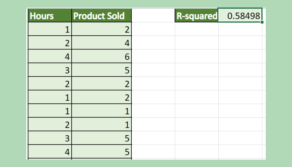
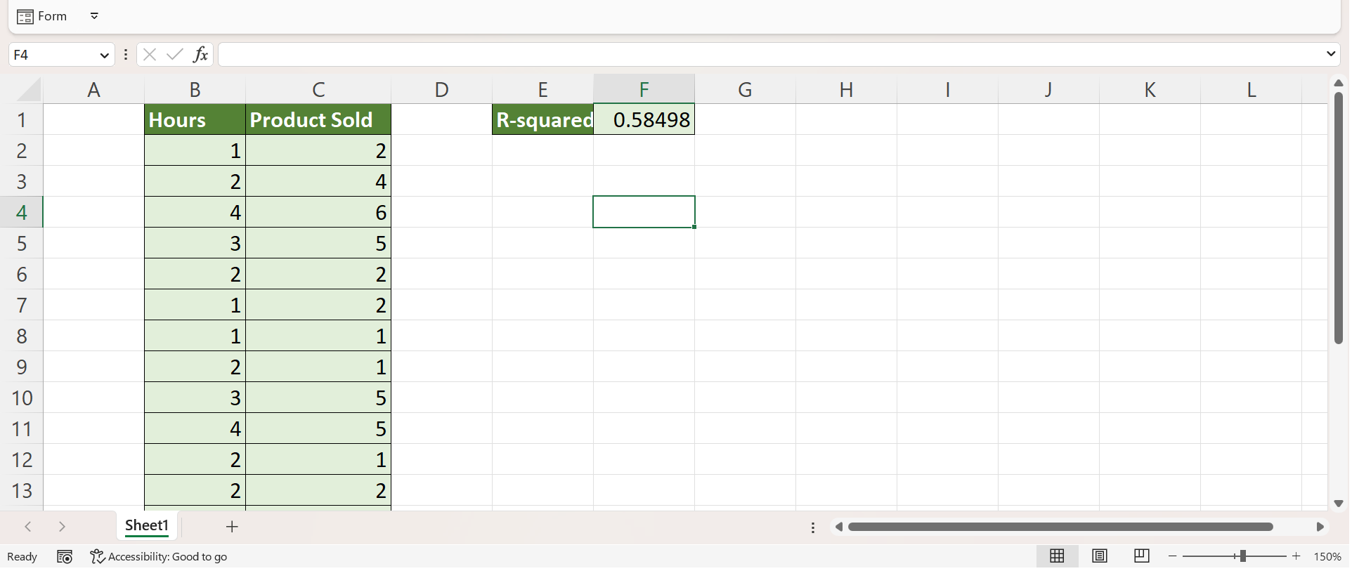
Let’s say we have the data for the number of hours an employee market to a customer and the number of products sold to a customer. So our initial data set would look like this:

And we want to fit a simple linear regression model to this data. Essentially, the R-squared refers to the proportion of the variance in the response variable that can be explained by the predictor variable.

In this example, our predictor variable is the number of hours, and our response variable is the number of products sold. However, the formula for finding the R-squared can be complex and prone to errors.  

Luckily, we can simply use the RSQ function in Excel to find the R-squared value of our data set. And the value for R-squared only range from zero to one. 

So a value of 0 can conclude that the predictor variable cannot explain the response value at all. Additionally, an r-squared value of 1 can mean that the predictor variable can completely explain the response variable without error. 

And we can simply use the RSQ function to calculate the R-squared value and determine the goodness of fit of our data set. So our final data set would look like this:

Based on the result, we have a 58.498% chance for the goodness of fit. Since the R-squared value is always in the range of 0.0 to 1.0 or 0% to 100%. With our result, we have a chance of our data values falling onto the regression line. 

Additionally, we can also fit a simple linear regression model to our data to verify whether our calculations are correct.

You can make your own copy of the spreadsheet above using the link attached below. 

Amazing! Now we can dive into the steps of calculating R-squared in Excel using the RSQ function.

How to Calculate R-squared in Excel

In this section, we will explain the step-by-step process of calculating the R-squared in Excel using the RSQ function. Furthermore, each step contains detailed instructions and pictures to guide you along the way.

1. Firstly, we need to calculate the R-squared value using the RSQ function. Next, we can simply type in the formula “=RSQ(C2:C21, B2:B21)”. Lastly, we will click the Enter key to return the result.

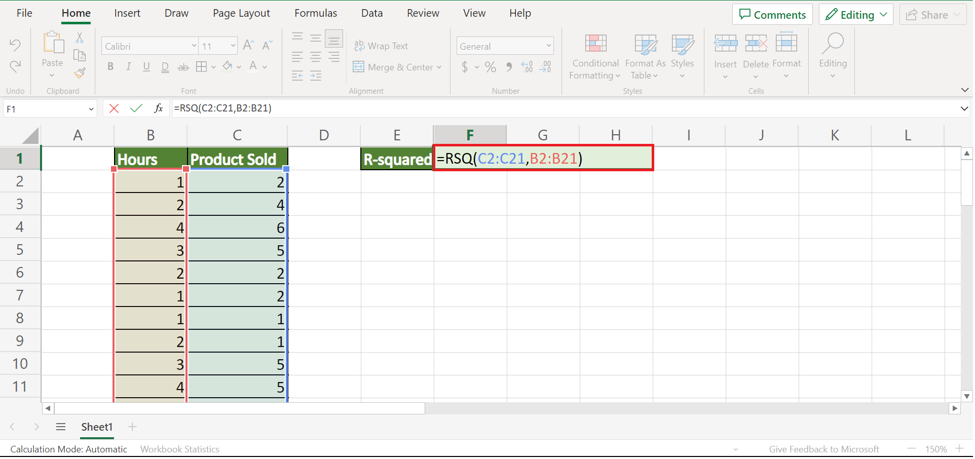
2. And tada! We have successfully calculated the R-squared value in Excel.

3. Additionally, we can fit a simple linear regression to verify our calculations. Then, we will go to the Data tab and select Data Analysis.

If you do not see this tool, you first need to install the free Analysis ToolPak.

4. Then, we will select Regression in the Data Analysis window. Lastly, we will click OK.

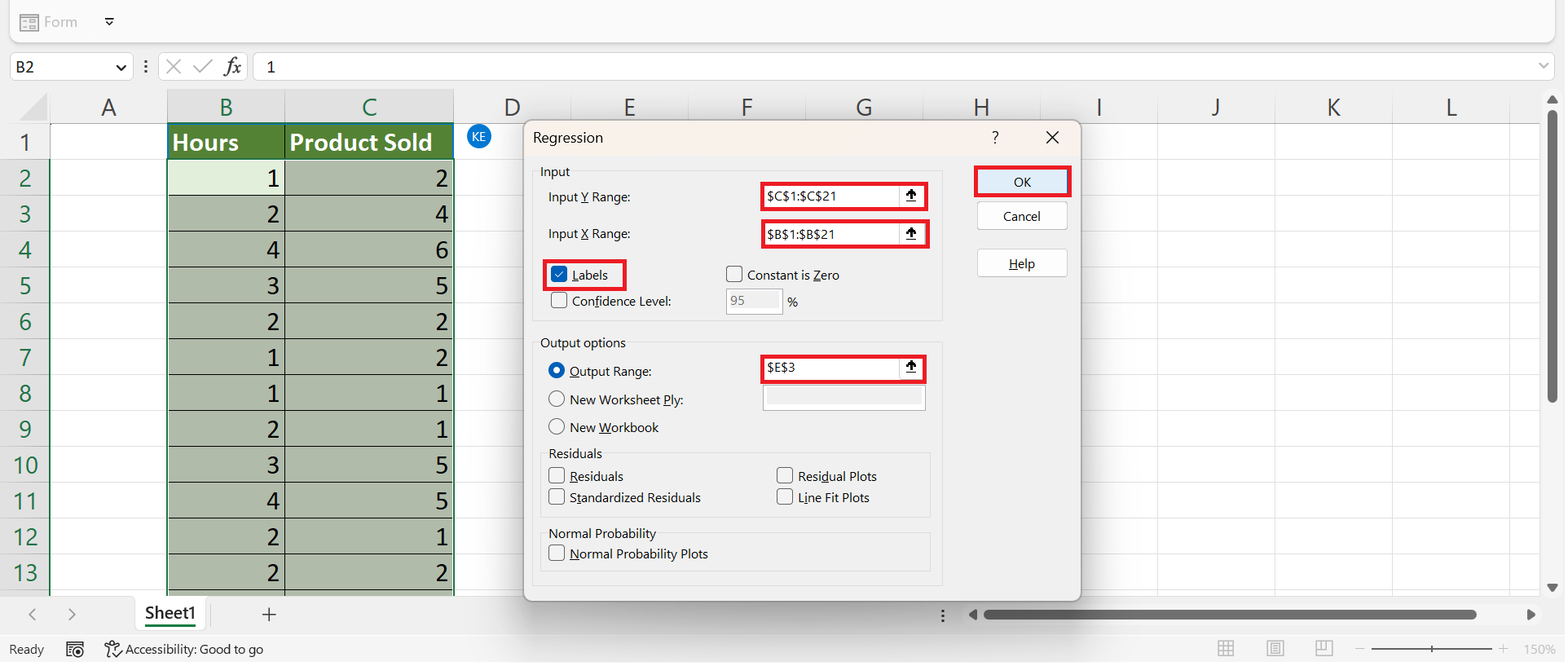
5. In the Regression window, we will select the response variable, which is the number of products sold for Input Y Range. Then, we will select the predictor variable, the number of hours for Input X Range. Next, we will check the box for Labels and select a cell to display the result for Output Range.

Lastly, we will click OK to apply all the changes.

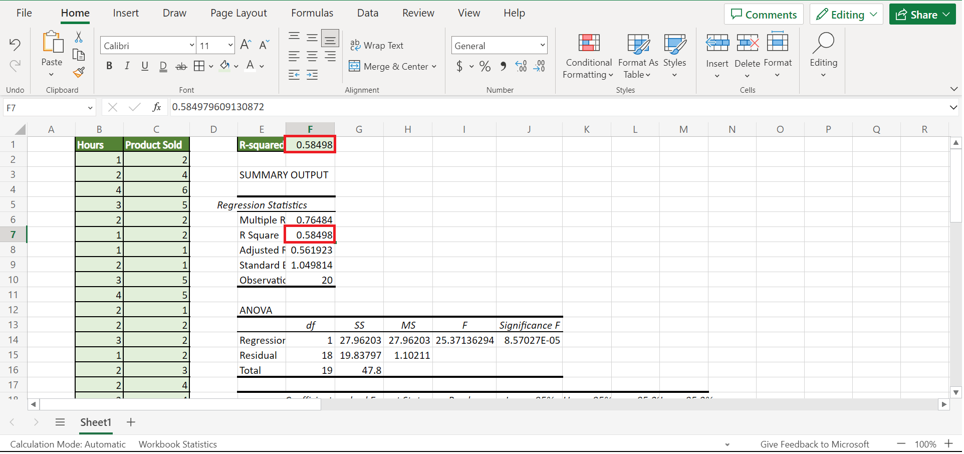
6. And tada! We have successfully displayed the summary output. In this summary, we can check whether we have the same value of R-squared using the RSQ function.

And that’s pretty much it! We have explained how to calculate the R-squared value in Excel using the RSQ function. Now you can apply this method whenever you need to find the R-squared.

Are you interested in learning more about what Excel can do? You can now use the RSQ function and the various other Microsoft Excel formulas available to create great worksheets that work for you. Make sure to subscribe to our newsletter to be the first to know about the latest guides and tutorials from us.

Get emails from us about Google Sheets.

Our goal this year is to create lots of rich, bite-sized tutorials for Google Sheets users like you. If you liked this one, you'll love what we are working on! Readers receive early access to new content.

Subscribe