How to Use LARGE Function in Excel

This guide will explain how to use the LARGE function in Excel.

We often need to find the largest or maximum value when working with datasets. However, there may be cases where you need to return the 2nd largest value, 10th largest value, and so on.

Microsoft Excel comes with a built-in LARGE function that allows us to return the nth largest element in a given dataset.

In this guide, we will provide a step-by-step tutorial on how to use the LARGE function in Excel. We’ll also cover other use cases that combine the LARGE function with other Excel functions.

The Anatomy of the LARGE Function

The syntax of the LARGE function is as follows:

=LARGE(data, n)

Let’s look at each argument to understand how the LARGE function works in Excel.

• LARGE() refers to our LARGE function. This function computes the nth largest element in a dataset.
• data refers to the array or range of cells to consider when returning the nth largest element.
• n refers to the rank (from largest to smallest) of the element to return. The value for n must be an integer from 1 to the size of the array or range provided.
• The formula LARGE(array, 1) will always return the largest element.
• If n is equal to the size of the range, LARGE(array,n) will return the smallest element.

A Real Example of Using the LARGE Function in Excel

Let’s explore a few basic examples that show how to use the LARGE function in Excel.

Using LARGE Function with Arrays 

Suppose we want to find the second largest value in the array {12,25,46,24,44,72,171}. 

We can input our array directly into the LARGE function as the first argument and set the second argument to 2.

We’ll use the following formula:

=LARGE({12,25,46,24,44,72,171},2)

After evaluating our formula, we find out that the second highest value in our array is 72.

Using LARGE Function with Cell Ranges

We can also use the LARGE function to find the nth largest value within a specific cell range.

In our example above, we have a dataset of 15 values in the range A2:A16. We want to find the fifth largest value in this range.

We can use the following formula to find the fifth-largest value in our range:

=LARGE(A2:A16,5)

After evaluating our formula, we’ve determined that the fifth largest value in our dataset is 737.

Using LARGE Function with Other Functions

We can also use the LARGE function with other built-in functions in Excel. In these cases, the LARGE function typically serves as a way to create criteria for other operations to use.

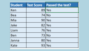
In the example shown, we used the  formula below to return “Yes” if the corresponding value in column A is one of the top 10 values of that range:

=IF(A2>=(LARGE($A$2:$A$16;10)),"Yes","")

The formula uses the LARGE function to find the 10th largest value in the range A2:A16. The IF function then compares the current cell to see if it’s greater than or equal to the 10th largest value. The IF function returns “Yes” if the condition is true and returns an empty string if false.

We can also use the LARGE function with a formula like SUMIF. For example, you may want to find the sum of the top 5 values in a particular range.

We can use the following formula to add the top 5 values in the range A2:A16:

=SUMIF(A2:A16,">="&LARGE(A2:A16,5))

To add just the top five values in the range, we’ll use the LARGE function to return the fifth largest number in the range. SUMIF will then use the criteria “>=”&LARGE(A2:A16,5) to ensure that we only add up numbers that are greater than or equal to the fifth largest number. In our example, we find out that the sum of our top five values is 4384.

In the example above, we used the LARGE function to help create a criteria argument that checks whether the value is greater than or equal to the fifth largest value before including it in the total.

Click on the link below to create your own copy of our examples.

Head to the next section to read our step-by-step tutorial on how to start using the LARGE function in Excel.

How to Use LARGE Function in Excel

1. Select the cell where you want to use the LARGE function.
   
2. Type the LARGE function and enter the two required arguments. The first argument should be the array or cell range that you want to find the nth largest value. The second argument should be an integer that determines the rank of the value you want to return.
   In the example above, our formula should return the largest value in the range A2:A16 since we set our rank to 1.
   
3. Hit the Enter key to evaluate the function.
   
4. We can set the range A2:A16 to a fixed absolute reference by typing it as “$A$2:$A$16”. This will allow the user to copy the formula down the rest of the column with the AutoFill feature.
   

FAQs

1. Why does the LARGE function return an error?
   If you are encountering a #NUM! Error, your n value may be higher than the number of values in the provided range, or the provided range does not contain any numerical values.
   
   
2. How do I return the smallest nth number in an array?
   If you want to find the nth smallest number in an array in Excel, you can use the SMALL function, which works similarly to the LARGE function but uses a reverse rank. Providing a rank of 1 will return the smallest number in the array.

To learn more about using the LARGE function, you can read our post on how it can be used alongside the VLOOKUP function in Excel.

That’s all for this guide! Be sure to check out our library of spreadsheet resources, tips, and tricks!