The UPPER function in Google Sheets is useful if you want to convert a given text to all capital letters.
Meaning, the UPPER function will help us convert texts into the uppercase format.
Table of Contents
The rules for using the UPPER function in Google Sheets are as follows:
- Texts that are directly passed to the UPPER function need to be enclosed with quotation marks.
- The argument can also be a cell reference containing the text that you want to be converted to all capital letters.
- Numbers and punctuation characters are not affected.
Let’s take an example.
Kaitlynn is tasked to clean up the data extracted from a third-party database. See some of the entries he received below:

Notice that some of the state and zip code entries are not in their usual format. This information is normally presented in all capital letters.
Instead of manually converting them, Kaitlynn applied the UPPER function to each item in columns B and C.

It saved her from doing the tedious work and she could now proceed to other things such as checking other columns to clean up.
Watch out for a more advanced tutorial and examples on how you can use the UPPER function in the coming weeks. Be sure to subscribe to be notified.
Awesome! Let’s begin getting to know more about our UPPER function in Google Sheets.
The Anatomy of the UPPER Function
So the syntax (the way we write) of the UPPER function is as follows:
=UPPER(text)
Let’s dissect this thing and understand what each of these terms means:
- = the equal sign is just how we start any function in Google Sheets. It is how Google Sheets understand that we are asking it to either do computation or use a function.
- UPPER() is our UPPER function. It converts text to all capital letters.
- text is the only and required argument in the function. This is the text that should be converted to uppercase.
A Real Example of Using UPPER Function
Let’s take a look at the data extracted by Kaitlynn below to see how the UPPER function is used in Google Sheets.

The UPPER function is pretty much straightforward. You need a text to be in all capital letters? Go ahead and pass it to the UPPER function and see the magic happens.
Let’s quickly analyze the first example. Formula in cell B2 used the cell A2 as its argument. This means that the UPPER function will convert the text ‘bc’, which is the state code of British Columbia in Canada, into its uppercase format, which is ‘BC’. The same applies to the remaining state codes from row 3 down to row 16.
Also, while texts in the state column are all letters, the texts in the zip code column are composed of letters and numbers.
Notice how the numbers in zip codes aren’t affected by the UPPER function.
Why is this so?
Well, that’s because the UPPER function only converts letters to uppercase format. Numbers and punctuation characters are ignored.

Like the PROPER function, the UPPER function above uses a cell reference, which contains the text to be converted into all capital letters.
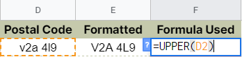
Furthermore, you can also pass a direct text as an argument to the UPPER function. See the example below:

Just don’t forget to enclose them with quotation marks so that the UPPER function would know that you are passing a string value.
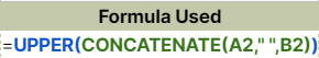
The UPPER function also processes an argument from a result of another function.

In the example above, the argument passed to the UPPER function is the resulting string of the CONCATENATE function.
Want to get to know more about the CONCATENATE function? Keep an eye out and be sure to subscribe to be notified as an article about it is underway.
The CONCATENATE function above joined three items. These are the text in cell A2, a space, and the text in cell B2. Note that the texts in cells A2 and B2 are not in the uppercase format.
The result is the string ‘roderick timbal’, which is the text that the UPPER function will then convert to all capital letters.
You may make a copy of the spreadsheet using the link I have attached below.
How to Use UPPER Function in Google Sheets
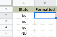
- Click on any cell to make it the active cell. For this guide, I will be selecting B2, where I want to show the result.
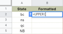
- Next, type the equal sign ‘=‘ to begin the function and then follow it with the name of the function, which is our ‘upper‘ (or ‘UPPER‘, not case sensitive like our other functions).

- Type open parenthesis ‘(‘ or simply hit Tab key to let you use that function.
- Now the exciting part! Let’s give our function its only argument, the text. You may pass constant data by typing the exact text after the parenthesis. Just don’t forget to enclose it with quotation marks (“”). In this case, type in ‘bc’.
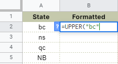
- Hit your Enter or Tab key. Cell B2 will now show you the uppercase format of the text provided.

- Notice that in this example, we provided the exact string value, constant, as the argument of our UPPER function. Alternatively, this constant can be a variable or simply a cell address containing your text.
- Edit the formula in cell B2 by changing the argument into the cell address, where your text to be converted to all capital letters is located. In this case, cell A2.

- Hit your Enter or Tab key again. Cell B2 will now show you the same result, which is the uppercase format of the text in cell A2.

- Copy the formula down to the remaining rows.

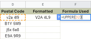
- Now, let’s do the same to the zip codes.
- On cell E2, repeat steps 1-4. For step 4, instead of the exact text value, we will pass the cell address to the UPPER function. Type in ‘D2’.

- Hit your Enter or Tab key. Cell E2 will now show you the uppercase format of the zip code in cell D2.
- Copy the formula down to the remaining rows.

- Columns B and E should now have the uppercase format of the texts in columns A and D.
That’s pretty much it. You can now use the UPPER function in Google Sheets together with the other numerous Google Sheets formulas to create even more powerful formulas that can make your life much easier.