How to Use HSTACK Function in Google Sheets

This guide will explain how to work with the HSTACK function in Google Sheets.

If you are dealing with data sourced from several tables or sheets, you might encounter a situation where you must combine data horizontally into a single table.

We can append ranges horizontally by using curly braces in our formula. For example, we can append the ranges A2:E5 and D7:E10 together using the formula ={A2:E5,D7:E10}.

In early 2023, Google Sheets released a new function called HSTACK, allowing you to append ranges horizontally into a larger array.

This guide will explain how to start using the HSTACK function in Google Sheets. We will cover how to use the function to append ranges horizontally. We will also explain how to handle cases where the appended ranges have a different number of rows.

Let’s dive right in!

The Anatomy of the HSTACK Function

The syntax of the HSTACK function is as follows:

=HSTACK(range1, [range2, …])

Let’s look at each term to understand how to use the function.

• = the equal sign is how we start any function in Google Sheets.
• HSTACK() refers to our HSTACK function. This function allows us to append ranges horizontally and in sequence.
• range1 refers to the first range to append to the new array.
• [range2, …] refers to all additional ranges we want to append to the new array.

A Real Example of Using the HSTACK Function in Google Sheets

Let’s explore a simple example where we may need to append two or more ranges horizontally with the HSTACK function.

In the table seen below, we have sales data for three different products. The data is separated into two sections: one for Q1 (January to March) and another for Q2 (April to June).

We want to create a new table that includes sales data from both quarters.

We can generate the table above by placing the following formula in cell A10:

=HSTACK(A1:D4,B6:D9)

The HSTACK function can also handle appending ranges with a different number of rows.

We can use the HSTACK and IFERROR functions together to fill in the cells with missing data:

=IFERROR(HSTACK(A1:D4,B6:D10),"0")

Do you want to take a closer look at our examples? You can make your own copy of the spreadsheet above using the link attached below. 

If you’re ready to try appending ranges horizontally, head over to the next section to read our step-by-step breakdown on how to do it!

How to Use the HSTACK Function in Google Sheets

This section will guide you through each step needed to begin using the HSTACK function in Google Sheets.

Follow these steps to start appending ranges horizontally:

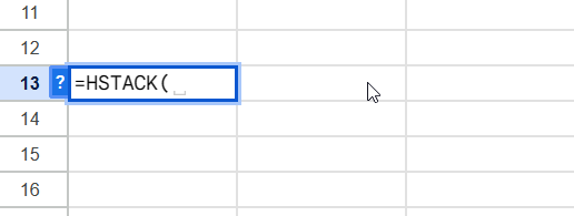
1. First, select an empty cell in your spreadsheet and type out the HSTACK function.
   
2. Specify the first range you want to include in the final array as the first argument of the HSTACK function.
   
   
   In our example, we have two tables that track sales in different quarters. We want to append these tables horizontally into a single table.
   
3. Next, we’ll add another argument to our HSTACK function. The second argument should include the range you want to append to the first argument.
   
   
   Users should note that the chosen ranges appear in the final array in the order they appear in the function’s arguments.
   
4. Hit the Enter key to evaluate the function. You should now have a new larger array that appends the two selected ranges horizontally.
   
5. The HSTACK function can support ranges with a different number of rows. The final array will have the same number of rows as the range with the most rows. The cells that lack additional cells are filled with a #N/A error.
   
   
   In the example above, we append two tables into a single array. However, since the data from the first quarter does not have a fourth column for Product D, our function returns #N/A errors to fill in the missing values.
   
6. We can replace the #N/A error with our own custom values. We’ll just need to wrap our HSTACK function with an IFERROR function.
   
   
   For example, we can catch the #N/A error and replace the missing values with 0.

Frequently Asked Questions (FAQ)

Here are some frequently asked questions about this topic:

1. 1. What is the difference between the HSTACK and VSTACK functions?
      The HSTACK function combines ranges horizontally. This means that the second range will appear to the right of the first range mentioned. The VSTACK function, however, appends data vertically. All newly appended data will appear below the previous argument.
   2. Why should you use HSTACK function rather than the curly braces method?
      The HSTACK function is a more user-friendly method since it already provides arguments for the user to fill out. The HSTACK function also allows you to combine ranges with a different number of rows.
      If we tried to append ranges with a different number of rows using the curly braces method, our formula would result in a #VALUE! error.

This tutorial should cover everything you need to know about the HSTACK function in Google Sheets.

We’ve tackled how to use the HSTACK function to append ranges horizontally. We’ve also explained how to handle #N/A errors that occur when the tables being appended have a different number of rows.

The HSTACK function is just one of many useful built-in functions in Google Sheets. If you found this guide helpful, you may be interested in reading our guide on how to combine two query results in Google Sheets.

You may also check our guide on how to use the IMPORTRANGE function in Google Sheets to learn how to work with data from multiple live spreadsheets at once.

That’s all for this guide on the HSTACK function! If you’re still looking to learn more about Google Sheets, be sure to check out our library of Google Sheets resources, tips, and tricks! 

Get emails from us about Excel and Google Sheets.

Our goal this year is to create lots of rich, bite-sized tutorials for spreadsheet users like you. If you liked this one, you'd love what we are working on! Readers receive early access to new content.

Subscribe