How to Use IFS Function in Google Sheets

The IFS function in Google Sheets is useful if you want to evaluate a set of expressions and value pairs without having too many nested values.

The IFS function is also helpful when we have to assess multiple expressions in sequence, and returns the first value for which expression is true. It’s as if helping us decide using the if-else-then structure.

Let’s take an example to better understand the IFS function.

Say I have a class with 50 students. In every grading period, I have to evaluate them using grades. However, our school only understands the letter grade system (A, B, C, D, and F). I want to easily convert numeric grading to the letter grade format. How should I do it?

It’s simple. We can use the IFS function and let it work its magic. Supply the function with expressions and do this by taking the numeric grade and test whether it’s greater than, less than, or equal than the value that we have as a standard (e.g. A1 > 85, “B+”). This expression would mean that if cell A1 is greater than 85, which is our standard, then it would result in the grade ‘B+’.

That’s how easy it is!

Let’s go into the real example where we will now use actual values and how we write our own IFS function in Google Sheets to compute those values.

The Anatomy of the IFS Function

So, the way we write the IFS function is:

=IFS(condition1, value1, [condition2, ...], [value2, ...])

Let’s break this syntax down to better understand each attribute:

• = the equal sign is just how we start any function in Google Sheets.
• IFS is our formula. We just have to add expressions which are basically conditions and corresponding values for it to work.
• condition1 is the first logical test.
• value1 will be our desired outcome for condition1 in case it turns out to be true.
• condition2, value2 – this is optional, and this is the second logical test and desired outcome. We can keep adding conditions and values without any limits.

⚠️ Now a few notes when you write your IFS Function.

1. You can use comparison operators like > for greater than, < for less than, and = for equal, in making your expressions.
2. The numbers are not enclosed in a quote-unquote (“”) symbol, while texts are.
3. There’s no way to set a default answer if all conditions/tests return “false”. In this case, you have to enter “true” in the last condition.
4. The IFS function returns an “#N/A” error if no conditions return “true“.

It may seem confusing up to this point, but I’ll assure you that after reading this guide, you will surely feel comfortable applying the IFS function in Google Sheets.

A Real Example of Using IFS Function

Take a look at the example below to see how the IFS function is used in Google Sheets.

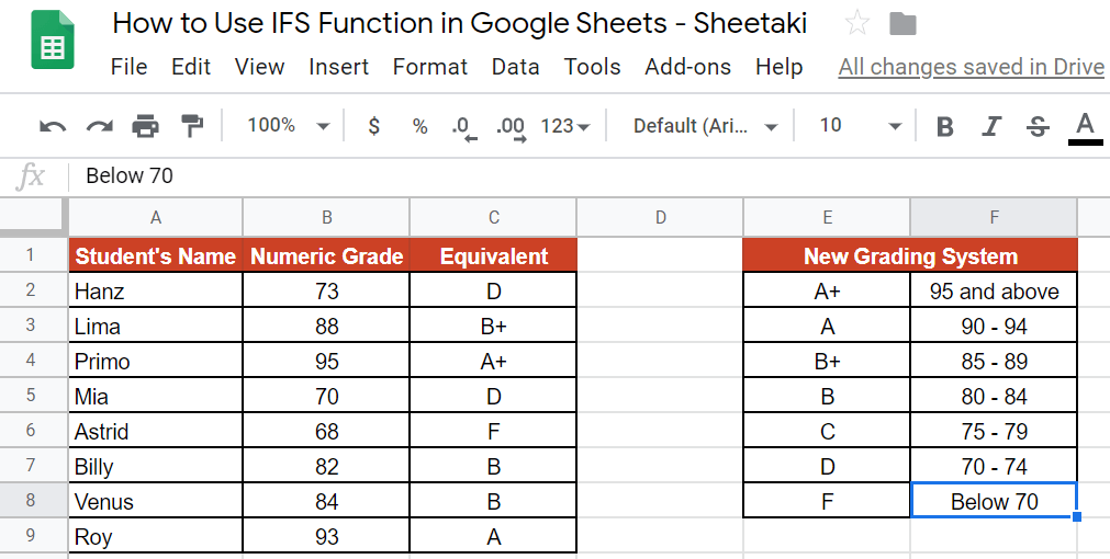
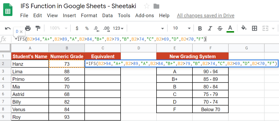
The example above shows how we used the IFS function to convert the numeric grade into the new grading system, which is the ‘grade’. Here, the IFS function can help us do the job because instead of manually inputting the letters, with a single formula, you can already transform each numeric grades in seconds!

The function is as follows:

=IFS(B2>94,“A+”,B2>89,“A”,B2>84,“B+”,B2>79,“B”,B2>74,“C”,B2>69,“D”,B2<70,“F”)

Here’s what this example does:

• First, we made a cell active. This is where we will write our IFS formula. For this guide, we selected cell C2.
• Next, we started off our formula with an equal sign, followed by our function, IFS.
• After that, we added our conditions. Since we already have our “New Grading System” guide, we will have to identify which statement would make each condition true or false.
• We used the symbols greater than “>” and less than “<” to denote the conditions.
• We dragged the formula down to C9.

See how simple was that! In just seconds, we were able to convert the numeric grades into letter grades.

You may make a copy of the spreadsheet using the link I have attached below:

Have a feel on how to work with this formula. Try it out for yourself.

Let’s begin writing our own IFS function in Google Sheets.

How to Use IFS Function in Google Sheets

So, we are already given a standard, as shown in the table beside the table of the students with their corresponding numeric grades.

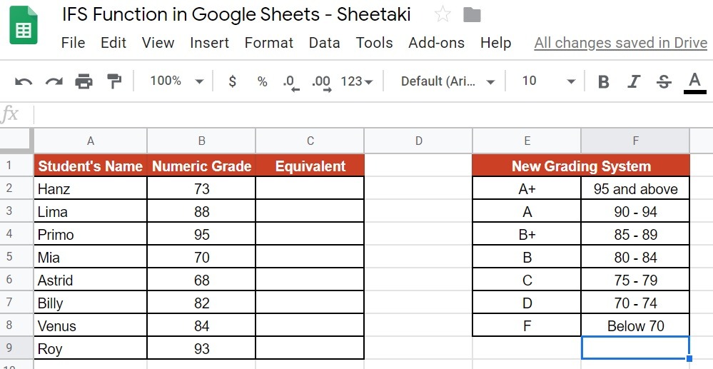
This standard will serve as our “legend” or guide in building our expressions. 🙂

1. Right after pre-determining the standard, the first step to writing our formula is to click on any cell to make it active. This is where we will write our formula. For this guide, I will be selecting the cell C2.

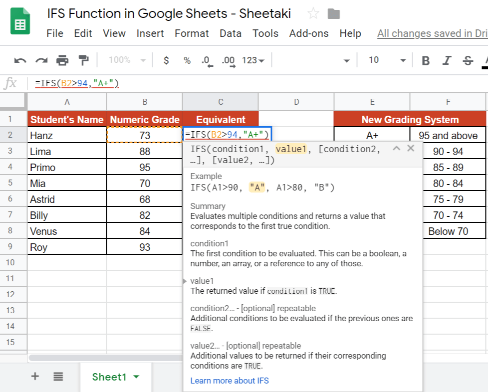
2. Next, on C2, we will start our formula with an equal sign (=), followed by the name of our function, which is IFS, then an open parenthesis ‘(‘. Wait for an auto pop-up message that contains the syntax, its summary, and the definition of its attributes. This will be your guide as you continue writing your formula.

3. As you can see in our standard, ‘New Grading System’, we have seven grades. Therefore, we expect to have the same number of expression, as well. To do the first expression, we have to click on the cell/data that we wanted to check. For this guide, we will click B2.

4. After this, we identify our comparison operator. Note that for the first item in the New Grading System, it says that 95 and above is represented by an “A+” mark. In this case, we can say that if the cell B2 is greater than 94, therefore it’s an A+. Hence, we will write that expression as B2>94, “A+”. Remember to enclose the text string in a quote-unquote (“”) symbol.

5. Before adding the next expression, make sure to add a comma ‘,‘. For the second expression, the process is the same. But, instead of writing 94, we will use the second standard, which is 89, and the A grade. Add another comma for the 3rd expression.

6. You do the same process until the 7th expression (grade F).

7. The last expression is different. Since it’s telling us that F is for grades below 70, then, we can conclude that it’s 69 and below. Grade 69 is lesser than 70. Hence, you should change the comparison operation to <. This would be your last step, so close the formula with a close parenthesis ‘)‘.

8. Lastly, hit the Enter key, then drag the formula down to cell C9 and be amazed!

That’s it. Well done! 👏🏆

You can now use the IFS function together with the other numerous Google Sheets formulas to create even more powerful formulas that can make your life much easier. 🙂

Get emails from us about Google Sheets.

Our goal this year is to create lots of rich, bite-sized tutorials for Google Sheets users like you. If you liked this one, you'll love what we are working on! Readers receive ✨ early access ✨ to new content.

Subscribe