Learning how to ignore blanks when calculating the weighted average in Microsoft Excel is useful when you want to calculate the weighted average of a wide range of data with empty cells.
Table of Contents
The weighted average function is more extensively employed in statistic calculation than the simple average. However, do you know the difference between a weighted average and a simple average?
All numbers are regarded identically and given equal weight when calculating a simple average, also known as an arithmetic mean. On the other hand, a weighted average provides weights that establish the relative value of each data point in advance.
The most common use of a weighted average is to equalize the frequency of values in a data set. For instance, a survey may collect enough responses from every age group to be statistically valid.
However, according to their population share, the 20-25 age group may have fewer respondents than the other age groups. The research team may weigh the results of the 20-25 age group to ensure that their perspectives are well-reflected.
However, values in a data set may be weighted for reasons other than the number of events. If students in an acting class are rated on skill, attendance, and etiquette, the skill score may carry more weight than the other aspects.
Now that you understand what weighted average is, let’s look into how we can calculate weighted average in Microsoft Excel.
We will use the SUMPRODUCT function and the SUM function to calculate the weighted average. However, to ignore the blank cells in Excel while calculating the weighted average, we use only the SUMPRODUCT function and other Excel elements.
Not to fear! Let’s understand how to convert and transform these formulas to calculate weighted averages while ignoring blank cells.
Anatomy of the SUMPRODUCT Function
The main function used to calculate the weighted average is the SUMPRODUCT function.
The sum of the products of related ranges or arrays is returned by the SUMPRODUCT function. Multiplication is the default operation, but addition, subtraction, and division are also available.
The SUMPRODUCT function has the following syntax:
=SUMPRODUCT(array1, [array2, array3, …])
Let’s take a closer look at each term in the formula to see what they mean:
=is the equal sign we use to start any function in Microsoft Excel.SUMPRODUCT()this is our SUMPRODUCT function. For the function to work, we’ll need to insert one or more arrays.array1is the initial array argument for which you want to multiply and then add the components.array2is the component you want to multiply and then add.
Usage of (–) in an Excel Formula
(–) converts a TRUE return value to 1 and a FALSE return value to 0. It has no bearing on the outcome. It’s usually used in conjunction with logical functions to transform Boolean type results to 0 or 1 form.
It’s often utilized with the SUMPRODUCT function in Excel to help ignore non-numeric data.
Usage of <> in an Excel Formula
The symbol <> in Excel stands for “not equal to.” The <> operator in Excel compares two values to see if they are equal.
If two cells are equal, the <> operator will return FALSE, but if two cells are not equal, the formula will return TRUE.
Are you overwhelmed? Do not worry! We will go through step-by-step how to combine these functions in a formula to calculate the weighted average while ignoring blank cells in Microsoft Excel.
A Real-Life Example of Calculating the Weighted Average While Ignoring Blank Cells
Let’s look at a real-life example of ignoring blanks when calculating the weighted average in Excel.
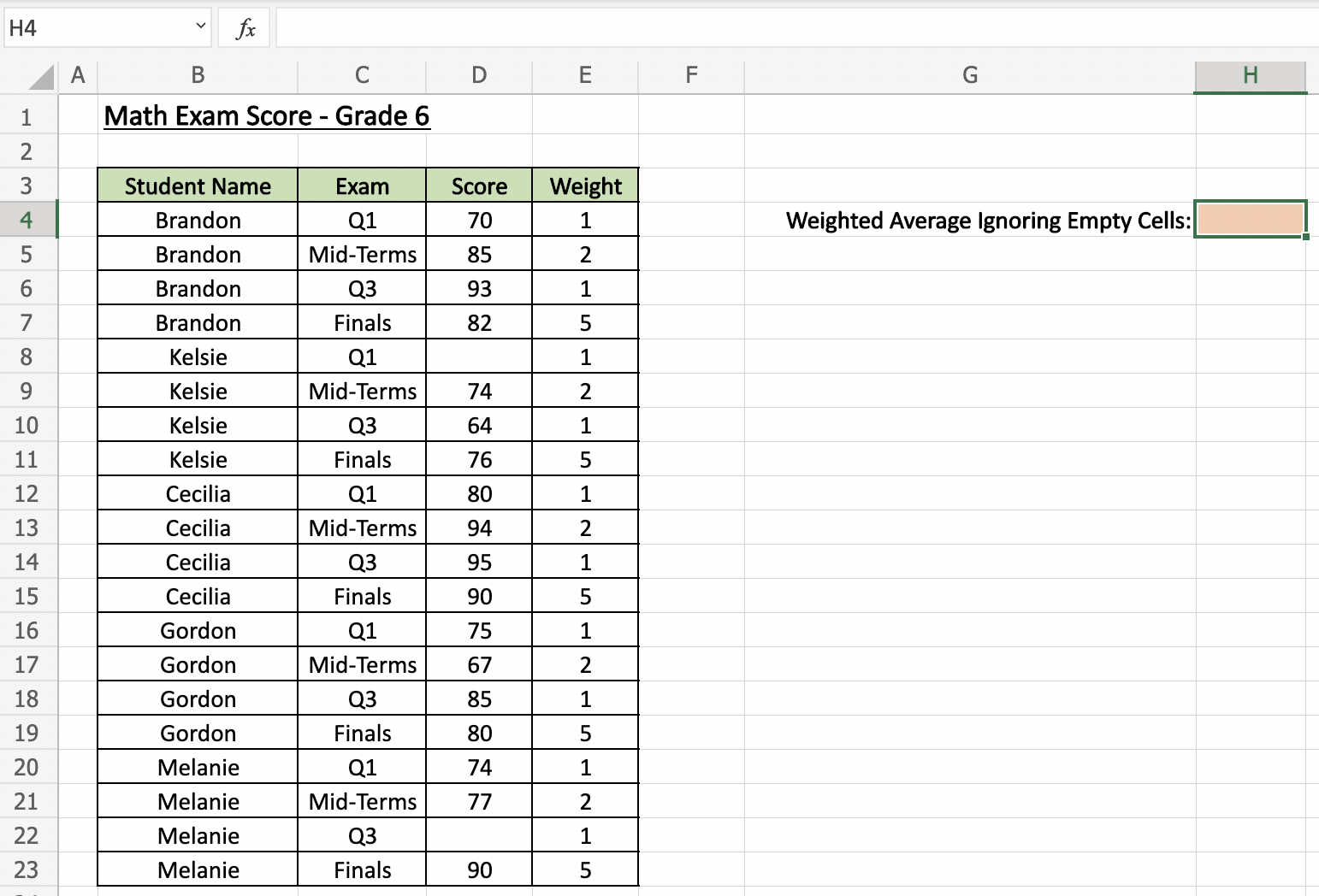
In this example, imagine you are a teacher for Grade 6. It is the end of the year, and you are required to create a report on the weighted average mark for all subjects for the entire Grade 6 students.
Each exam is weighted differently as the Mid-terms and Finals are weighted more heavily than the Q1 and Q3 exams.
While most of the students attended all exams during the year, some were absent. This has resulted in some cells being empty while recording the data of the entire Grade 6’s math exam scores.
By using the formula shown below, you can calculate the weighted average of the Math Exam score for the entire Grade 6 students.
You may make a copy of the spreadsheet using the link I have attached below.
Once you are ready and understand all the functions involved, we can jump into writing the formula together!
How to Ignore Blanks When Calculating the Weighted Average in Excel
This section will walk you through each step of finding the weighted average in Microsoft Excel while ignoring blank cells.
Follow these steps to start calculating the weighted average while ignoring blank cells:
- First, let’s select the cell we want to key our formula in. In this example, we will select H4 to type the formula.
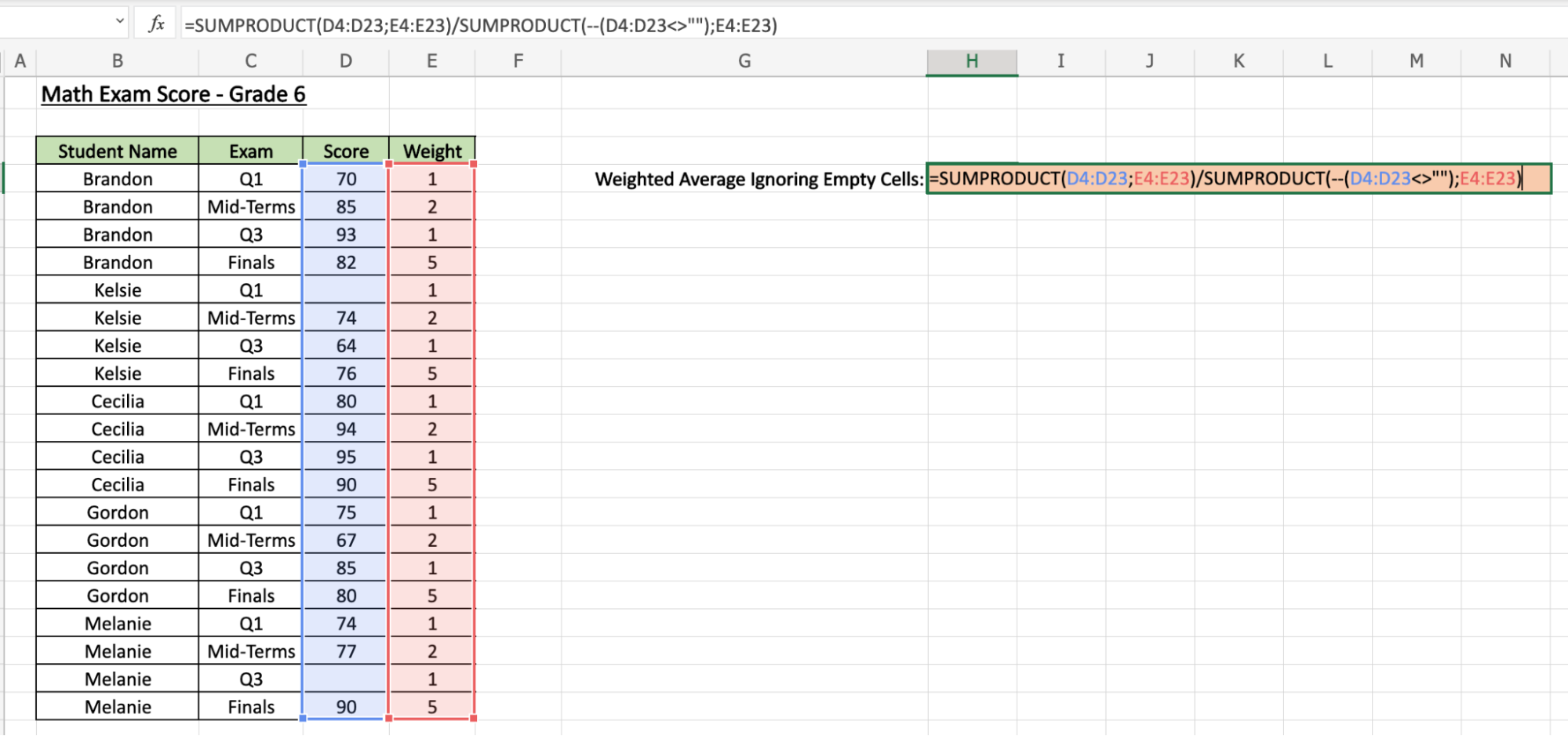
- Next, we insert the equal sign
=to begin the function, followed bySUMPRODUCT(.

- Then, we select the array of scores and the array of weights allocated to each test. In this case, it is D4:D23 followed with a semicolon
;and select E4:E23. Don’t forget to close the first formula by inserting a close parentheses).

- Next, we type in this formula
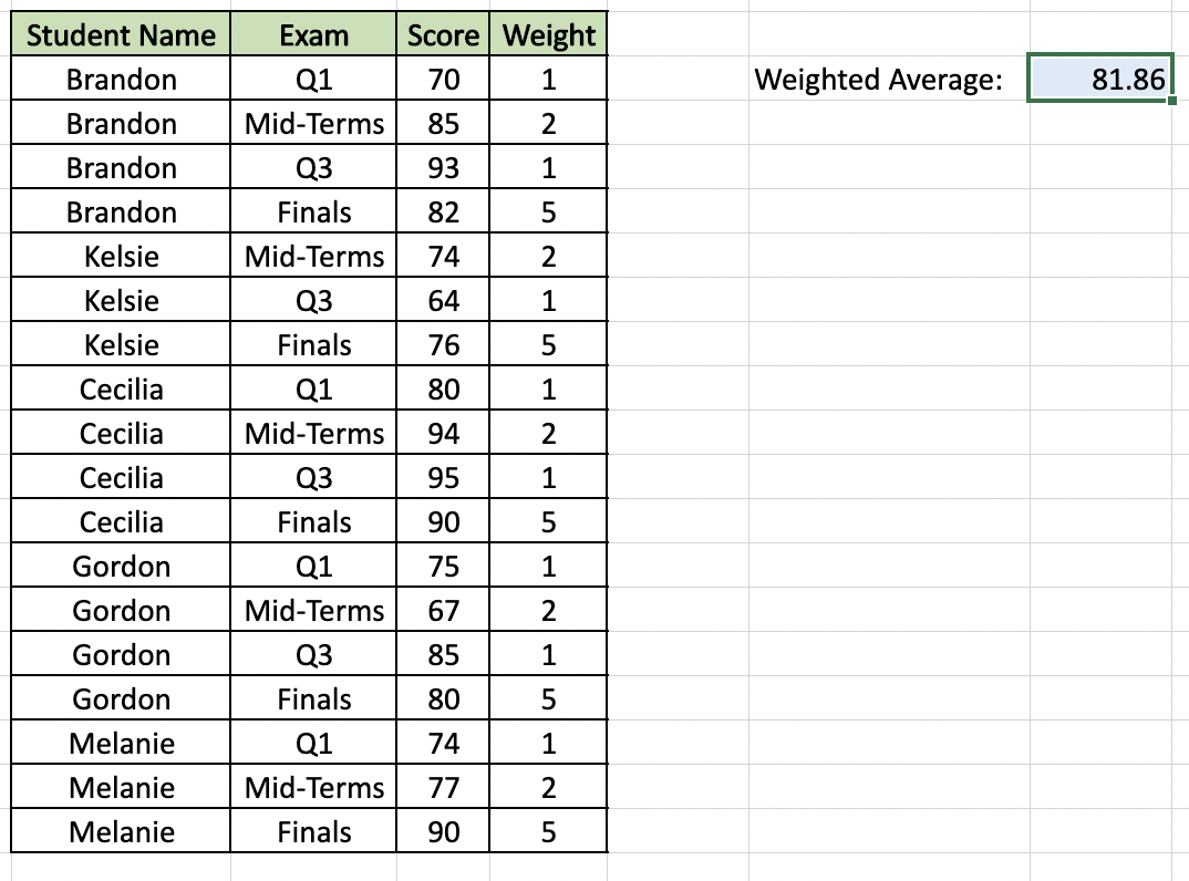
SUMPRODUCT(--(D4:D23<>"");E4:E23).
- Once we press Enter, the weighted average calculated will be 81.86.
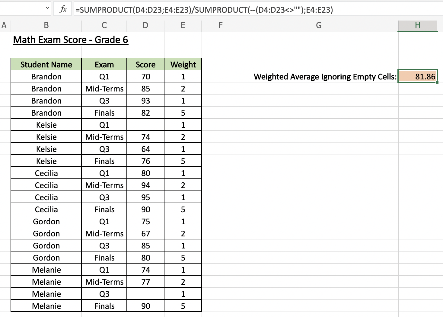
Let’s look closer into the formula and dissect how each function played a role.

So, what the formula did was, to sum up all the weights but ignored those blank cells.
To confirm that this formula is accurately performed, we can calculate the weighted average of the same data but remove the blank cells.
There you go! Now you know how to calculate the weighted average in Microsoft Excel while ignoring the blank cells.
Don’t forget to check out other cool functions in Microsoft Excel to enhance and simplify work for your everyday use!
Make sure to subscribe to our newsletter to be the first to know about the latest guides and tutorials from us.