How to Use ISBLANK Functions in Google Sheets

The ISBLANK function is useful if you want to find out whether a cell is empty.

Let’s take an example.

Say we have a cell or box (whatever you call those square-things in your spreadsheet) and let’s also say the cell has a value in it.

You want to find out whether the cell is really empty.

Well, you could just manually figure it out as any sane person would do, but there is a way to let the spreadsheet handle it by itself.

Using the ISBLANK function, it can tell whether a value occupies the cell. Where when the value occupies the cell it will return False. If you were to remove the value from the cell, the cell will be empty and the function will return True since it is blank/empty.

This function works for any cell value type: numbers, text strings, formula, or even a formula error. Where and when if a value is present the function result would be false.

To really get the most out of this function, you can try it together with an IF function where you can carry out an action when a cell is empty or otherwise. For instance, taking the same value ‘8’ example from above, if the ISBLANK returns False then output the word ‘Apple’ into another cell using an IF function. This also works vice versa where when the cell is empty it returns True and using IF function you can output the word ‘Orange’ into a cell.

Great! Let’s dive right into real-business examples where we will deal with actual values and how we can write our own ISBLANK function in Google Sheets to automate our tasks.

The Anatomy of the ISBLANK Function.

There is a term to how we call writing a function and that term is called syntax. It’s pretty commonly used everywhere.

So the syntax (the way we write) the ISBLANK function is as follows:

=ISBLANK(value)

Let’s dissect this thing and understand what each of the symbols and terms means:

• = the equal sign is just how we start off any function in Google Sheets
• ISBLANK() this is our ISBLANK function. ISBLANK returns TRUE if the value is empty or a reference to an empty cell and FALSE if the cell contains data or a reference to data. We will have to add our value into it in order for the function to work.
• value is the reference to the cell that you will be checking for ‘emptiness’. The value can be just a single cell A2 or a range of cells A1:C10

Frequently Asked Questions (FAQ)

1. Many of our readers have to come to ask the question: Why ISBLANK returns FALSE even when the reference cell is empty? This may sometimes be a bug from Google’s end but more often than not, it is because of us. One common instance is, say, when if we have a value in cell A1 that is “Donuts” and then the formula in B1 is as follows:

=IF(A1="DONUTS", "", "WRONG ENTRY")

Result: ""

You’ll find that the above formula returns a blank. Now, what happens if we were to use our newfound ISBLANK formula as shown below?

=ISBLANK(B1)

What do you think the result would be that will be returned by the ISBLANK formula?

Result: FALSE

You see, the value returned by the logical test in cell B1 (the IF formula above) is blank. However, our ISBLANK formula returns a FALSE because the blank cell is not actually blank. This is because of the "" even-though it may not be visible.

Hope you understand it. 😅

Similarly, if there are white space, beeline or any hidden characters, the ISBLANK formula would return FALSE only. So be cautious when you use the ISBLANK formula as a blank really means it’s completely blank without any transparent, hidden characters present. If there is, then clear the cell and try again.

2. Another question received from our readers was that How to test multiple blank cells in  Google Sheets? Pretty simple. The ISBLANK function can be used to check multiple cells at a time.

Here’s how you do it: Say we want to test the range of cells A1: A10 for blanks. Then simply use this range as a value in ISBLANK and then wrap the entire formula with the ARRAYFORMULA function.

=ARRAYFORMULA(ISBLANK(A1:A10))

You can also make the range as a multiple of columns at a time:

=ARRAYFORMULA(ISBLANK(A1:B10))

Now you may feel like you need to understand everything that I just wrote above, but don’t worry. We will go through it together and you will understand once you practice applying it, which we will be doing next.

A Real Example of Using ISBLANK Function

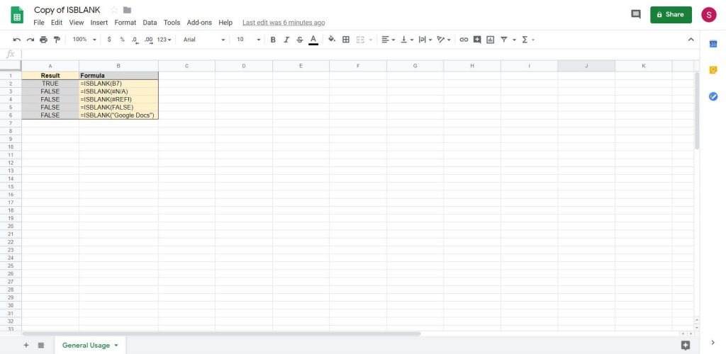
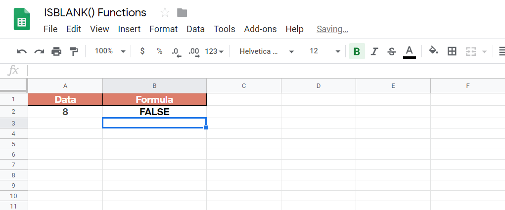
Take a look at the example below to see how ISBLANK functions are used in Google Sheets.

As you can see the result will be FALSE or TRUE when evaluated using the ISBLANK function.

You may make a copy of the spreadsheet using the link I have attached below:

Now, this is just the simplest examples of ISBLANK and does not really reflect real usage.

In real use cases, ISBLANK is useful in logical tests. For date-related calculations, ISBLANK is useful to find the difference between two dates.

Here’s an example formula

=IF(ISBLANK(A1), B1, A1-B1)

This formula simply means: return date in B1 if the date (or any value for that matter) is blank. Else, return the value of A1 minus B1. This IF–ISBLANK combo function allows you to skip blank cells for any calculations (date, numbers, etc)

You can try it out by yourself. 

Let’s begin writing our own ISBLANK function in Google Sheets.

How to Use ISBLANK Function in Google Sheets

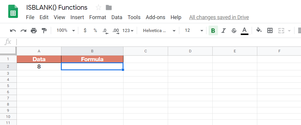
1. Simply click on any cell to make it the ‘active’ cell. For the purposes of this guide, I’m going to choose B2 as my active cell.

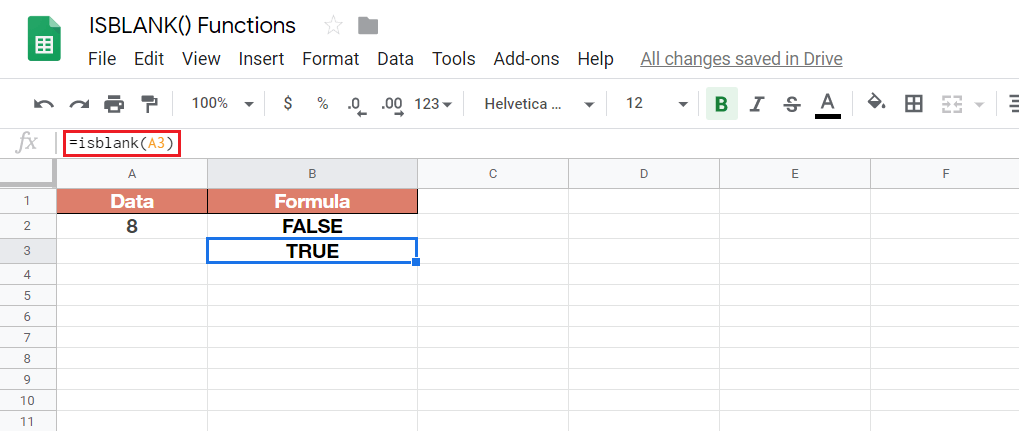
2. Next, simply type the equal sign ‘=‘ to begin the function and then followed by the name of the function which is our ‘isblank’ (or ‘ISBLANK‘, whichever works).

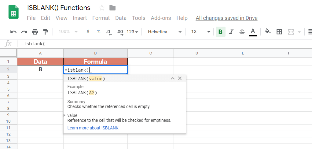
3. Now you should find that the auto-suggest box appears with the names of the functions that all are ISBLANK. Simply choose ISBLANK.

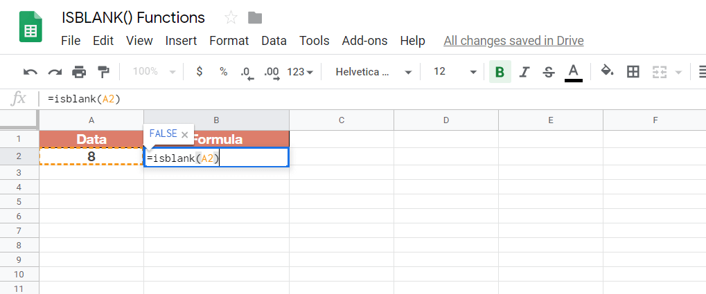
4. Great! Next, add in the value that you want to evaluate. I will be using A2 to find out if the value in A2 is blank or not. Whereby a TRUE or FALSE will be outputted. As you can the spreadsheet shows False (in the little box) as it already knows beforehand that it is False. Once you’ve entered the value (cell ‘A2‘ in my case), simply close the brackets of the function. Your function should now look somewhat similar to mine:

Tip: The cell (or box) you select has a fancy name called the cell reference which means that the cell is used as a reference for the function.

5. Finally just hit your Enter key. You’ll find that, if you followed my steps, that the value FALSE is output because A2 is not blank.

6. However, when I did similarly using the above cells in B3 to refer to cell A3 (to find out whether A3 was blank or not), it output TRUE because the cell is in fact blank.

That’s pretty much it. You can now use the ISBLANK functions inside IF functions or the other numerous Google Sheets formulas to create even more powerful formulas. 🙂

Get emails from us about Google Sheets.

Our goal this year is to create lots of rich, bite-sized tutorials for Google Sheets users like you. If you liked this one, you'll love what we are working on! Readers receive ✨ early access ✨ to new content.

Subscribe