How to Calculate P-Values in Google Sheets

You might need to calculate p-values in Google Sheets when you need to find out if there is a statistical difference between two samples. 

The p-value measures the probability that an observed test result could have occurred just by random chance or under the null hypothesis.

In this guide, we’ll show you when this type of calculation can be used. But first, let’s understand what the p-value refers to.

The p-value determines whether a hypothesis is true or not. We first define a certain threshold to consider the data as being correlated or not. This constant is known as the significance level. Usually, this is set to 0.05.

If the calculated p-value is below the significance level, then the expected results are considered statistically significant. A lower p-value means that your data is more likely to have a significant difference.

Let’s say you want to know whether there is a statistically significant difference between test scores found in a pre-test and post-test exam. We can use the T.TEST function to find the p-value of this hypothesis.

The function requires four arguments and follows the following syntax: 

TTEST(array1, array2, tails, type)

In the example described above, our two arrays would be the ranges of pre-test scores and post-test scores.

The tails argument refers to the number of tails used for the distribution. The type argument is an integer value that can refer to either a paired t-test (1), a two-sample equal variance t-test (2), or a two-sample unequal variance t-test (3).

This use case is just one example where p-values might be useful. Let’s learn how to use the T.TEST function ourselves in Google Sheets and later test out the function with an actual dataset.

Using T.TEST to Find the p-value in Google Sheets

Let’s take a look at an actual example of the T.TEST being used in a Google Sheets spreadsheet.
In the example below, we have a dataset of students and the following information: the scores of their pretest exam and the scores of their post-test exam.

Using the T.TEST function, we were able to find out that the P-value of the relationship between both variables is well below the 0.05 threshold. This indicates that there is a significant difference between both variables.

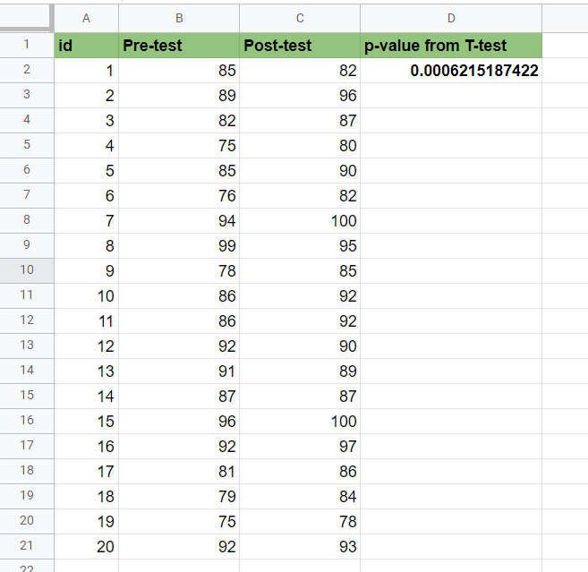
Since each pre-test result is paired with a corresponding post-test result, we should use a paired sample t-test. This type of test is useful when comparing the means of two samples, where each observation in a sample has a pair in the other sample.

To get the values in cell D2, we just need to use the following formula:

=T.TEST(B2:B21,C2:C21,2,1)

You can make your own copy of the spreadsheet above using the link attached below. 

As another example, let’s say we got two samples out of our pretest scores: x and y. Let’s see if there is a significant difference between their means.

The p-value returned is much higher than our threshold of 0.05, so we can say that there is no significant difference between these two samples. This is expected since their means should more or less be the same if they are both random samples from the same population.

If you’re ready to find the p-value on your own in Google Sheets, let’s proceed with the next section!

How to Use the T.TEST Function to get the P-Value

In this section, we will go through each step needed to start using the T.TEST function to find p-values in Google Sheets. We’ll use the pre-test and post-test exam score dataset found in the prior example.

Follow these steps to start using the T.TEST function:

1. First, select the cell which will hold the result of our T.TEST function.
   
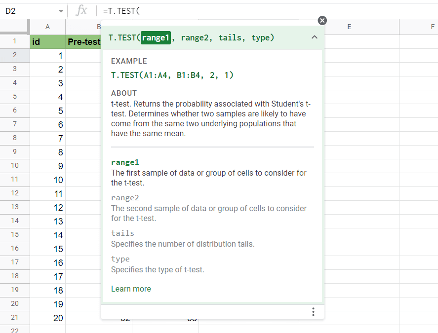
2. Next, we just simply type the equal sign ‘=‘ to begin the function, followed by ‘T.TEST(‘. 
3. After typing in the function name, you may find a tooltip box with hints on how to use the current function. We can click on the arrow on the top-right-hand corner to minimize if needed.
   
   
   
   
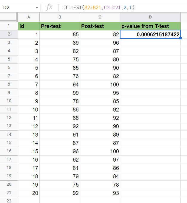
4. The next step is to type in our arguments. We will need the ranges B2:B21 and C2:C21 for our arrays. Since we’ll be needing a two-tail paired sample t-test, we’ll be using 2 as our tails argument and 1 as our type argument.
   Afterward, simply hit Enter on your keyboard to let the function evaluate.
   

Frequently Asked Questions (FAQ)

1. Why does my T.TEST formula return a #N/A error?
   Make sure that both of your array arguments are of the same length. If there is a shorter dataset, our T.TEST function will return a #N/A! error. 
2. Why does my T.TEST formula return a #NUM! error?
   Make sure that your tails argument is either 1 or 2 and that your type argument is equal to 1, 2, or 3.  
3. Why does my T.TEST formula return a #VALUE! error?
   If the tails or type argument contains non-numerical values, the T.TEST formula will return a #VALUE! error.

Using the T.TEST function is the easiest way to calculate p-values in Google Sheets. This step-by-step guide shows how simple it is to set up a t-test to determine whether variables in your dataset have any correlation.

The T.TEST function is just one example of a statistical function in Google Sheets. With so many other Google Sheets functions out there, you can surely find one that will help with your calculations.

Are you ready to learn more about Google Sheets? Make sure to subscribe to our newsletter to be the first to know about the latest guides and tutorials from us. 

Get emails from us about Google Sheets.

Our goal this year is to create lots of rich, bite-sized tutorials for Google Sheets users like you. If you liked this one, you'd love what we are working on! Readers receive ✨ early access ✨ to new content.

Subscribe