How to Perform VLOOKUP with Two Lookup Values in Excel

This guide will discuss how to perform VLOOKUP with two lookup values in Excel.

The rules for using the VLOOKUP function in Excel are the following:

• The VLOOKUP function is used to look for a value in the leftmost column of a data set. Then, the function will return a value in the same row from the specified column. 
• By default, the function will perform an approximate match.
• The function is not case-sensitive.
• The range_lookup argument will decide the match mode. If we want an exact match, we will input FALSE. Otherwise, or TRUE, the default is an approximate match.
• When the range_lookup is TRUE, 1, or omitted, the function will match the nearest value less than the lookup_value and will still use an exact match.  
• When the range_lookup is FALSE or 0, the function performs an exact match and column 1 of the table_array does not have to be sorted. 

Excel is an excellent tool to use for complex calculations and situations. Since it has several built-in functions and tools, we can easily manipulate our data set and perform difficult tasks.

For instance, we want to look up certain values in Excel. And we can easily do this using different functions, specifically the VLOOKUP function. However, there are times when we need to use more than one lookup value in the VLOOKUP function.

But, the VLOOKUP function does not support using multiple lookup values. Luckily, there are two simple ways we can go about this issue. Essentially, we will use a helper column and combine the two lookup values using the ampersand and the CONCAT function.

Let’s take a sample scenario wherein we must perform VLOOKUP with two lookup values in Excel.

Suppose we have an employee directory. And we want to extract the department for certain employees. However, the first name and last name of the employees are separated into two different columns. Thus, we need to use two lookup values.

To do this, we can create a helper column combining the first name and last name of the employees in one column. Then, we can use the VLOOKUP function and concatenate the two lookup values with the ampersand symbol (&). 

Before we move on to a real example of performing VLOOKUP with two lookup values in Excel, let’s first learn the syntax of the functions we will be using. 

The Anatomy of the VLOOKUP Function

The syntax or the way we write the VLOOKUP function is as follows:

=VLOOKUP(lookup_value, table_array, col_index_num, [range_lookup])

Let’s take apart this formula and understand what each term means:

• = the equal sign is how we activate any function in Excel.
• VLOOKUP() refers to our VLOOKUP function. And this function is used to return a value from the same row of the lookup value from a column we specify. 
• lookup_value is a required argument. So this refers to the value found in the data set’s first column. Additionally, this value can be a value, a cell reference, or a text string.
• table_array is another required argument. And this refers to a table of text, numbers, or logical values in which data is retrieved. 
• col_index_num is also a required argument that refers to the column number in the table_array from which the matching value should be returned. 
• range_lookup is an optional argument. And this is a logical value that defines the type of match to look for. If we want the exact match, we input FALSE. If we want the closest match, we input TRUE. 

The Anatomy of the CONCAT Function

The syntax or the way we write the CONCAT function is as follows:

=CONCAT(text1, …)

Let’s take apart this formula and understand what each term means:

• = the equal sign is how we start any function in Excel.
• CONCAT() is our CONCAT function. And this function is used to concatenate a list or range of text strings. 
• text1 is the only required argument. So this refers to 1 to 254 text strings or ranges we want to join to a single text string.

Great! Now we can dive into a real example of performing VLOOKUP with two lookup values in Excel.

A Real Example of Performing VLOOKUP with Two Lookup Values in Excel

Let’s say we have a data set containing the employees’ names and their departments. And each employee separates the first name and last name into two columns. So our initial data set would look like this:

Our goal is to return the department a specific employee belongs in using their complete name as the lookup value. However, the first name and last name are separated into two columns. Thus, we have to use two lookup values when we look for the department they belong in.

In this case, we will use the VLOOKUP function to look for the employee name and return the department of the matching value. Since the VLOOKUP function does not support two lookup values, we would have to concatenate the two lookup values into one. And there are two methods we can perform.

Firstly, we will create a helper column. In this helper column, we will combine the first and last names into one column. Then, we will use the VLOOKUP function and the ampersand (&) to combine the two lookup values in the formula. 

So the formula would utilize the helper column to find a match and successfully return the matching department.

Secondly, we will still use the helper column. However, this time we will use the CONCAT function together with the VLOOKUP function. So the CONCAT function will combine the two lookup values in the formula and look for a match in the helper column. Then, it will return to the matching department. 

So our final data set would look like this:

You can make your own copy of the spreadsheet above using the link attached below. 

Amazing! Now we can proceed to discuss the steps of how to perform VLOOKUP with two lookup values in Excel.

How to Perform VLOOKUP with Two Lookup Values in Excel

In this section, we will discuss the step-by-step process of how to perform VLOOKUP with two lookup values in Excel.

1. Firstly, we need to create a helper column. To do this, we will insert a new column on the leftmost side of the data set. Next, we will type in the formula “=B2&C2” to combine the two lookup values.

2. Next, we will drag the Fill Handle tool to copy the formula to the rest of the cells.

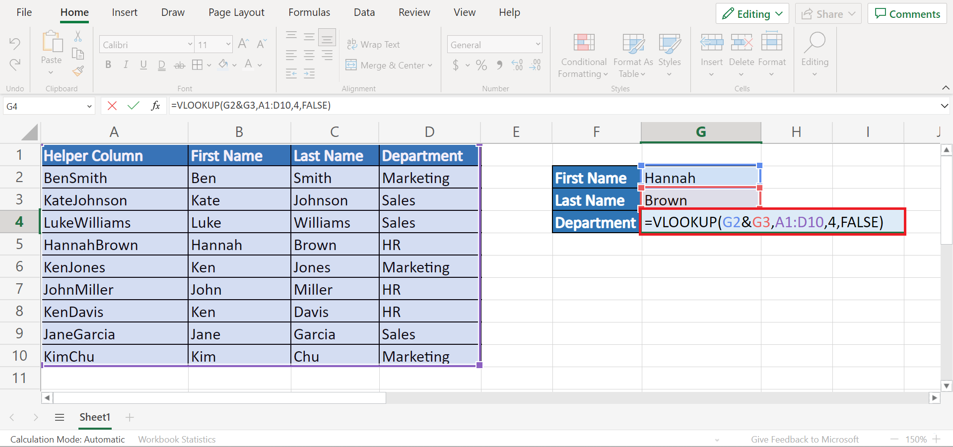
3. Then, we can create an area to input the lookup values and return the result. And now we can try our first method using the ampersand (&) symbol. To do this, we will input the formula “=VLOOKUP(G2&G3, A1:D10, 4, FALSE)”. Lastly, we will press the Enter key to return the result.

4. Afterward, let’s try our second method using the CONCAT function. To do this, we will type in the formula “=VLOOKUP(CONCAT(G2, G3), A2:D10, 4, FALSE)”. Lastly, we will press the Enter key to return the result.

5. And tada! We have successfully performed VLOOKUP with two lookup values in Excel.

And that’s pretty much it! We have discussed how to perform VLOOKUP with two lookup values in Excel using two easy and simple methods. Now you can choose one and apply it to your work. 

Are you interested in learning more about what Excel can do? You can now use the VLOOKUP function and the various other Microsoft Excel formulas available to create great worksheets that work for you. Make sure to subscribe to our newsletter to be the first to know about the latest guides and tutorials from us.

Get emails from us about Google Sheets.

Our goal this year is to create lots of rich, bite-sized tutorials for Google Sheets users like you. If you liked this one, you'll love what we are working on! Readers receive ✨ early access ✨ to new content.

Subscribe