How to Sum Every N Cells to the Right or Bottom in Google Sheets

The circumstances of adding up every n cells in Google Sheets are countless.

We may obsessively use the SUM function to add values instantly. But, in this guide, you will learn how to use the SUM() function to sum up every n cells to the right or bottom in Google Sheets.

Let’s take, for instance, you have a quarterly record of your sales, and at the end of every quarter, you’d want to check how many sales did you make. Another, if you wanted to do an inventory count semi-annually, and you’d want to know how many of X items are left. Or maybe, you have to see how much are your expenses for each category each month.

Those are just a few of the many scenarios that we can sum every n cells in Google Sheets.

Using the SUM function, we can actually pair it with other functions so we can achieve today’s learning goal: To sum every n cells to the right or bottom in Google Sheets.

In this guide, we will be having two examples to show you exactly how to sum every n cells to the right and to the bottom step-by-step.

The example we will be going over is to try and check our quarterly sales for the year 2019. We are given a per month sales value and we require to sum up for each quarter (every three months). You will understand more as you read on. 🙂

Let’s jump right in!

How to Sum Every N Cells to the Right in Google Sheets: 10 Steps

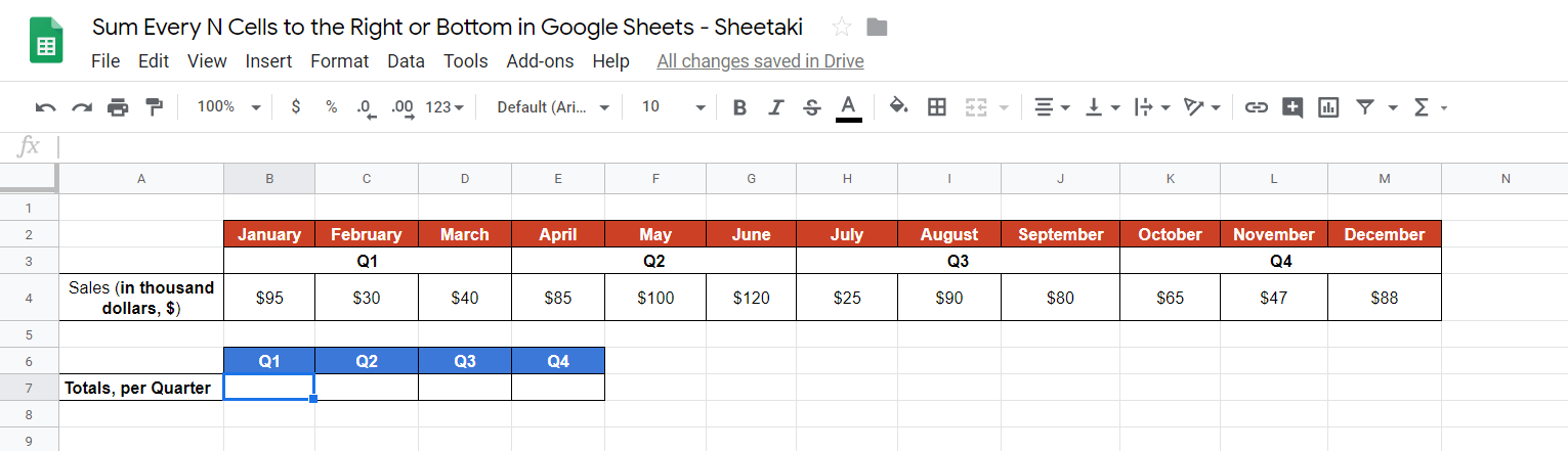
1. Jump into your Google Sheets and enter your monthly sales in a horizontal manner. The value can be in units or in monetary figures ~ your pick. In this example, we will have them in dollar amounts. For this guide, I have placed the labels, Q1 to Q4, for easier reference in the next steps.

2. Done inputting your sales? Good job! Now that your monthly sales are there, let’s now click on any cell and make it active. This is where we will write our formula. For this guide, I’ll be selecting B7.

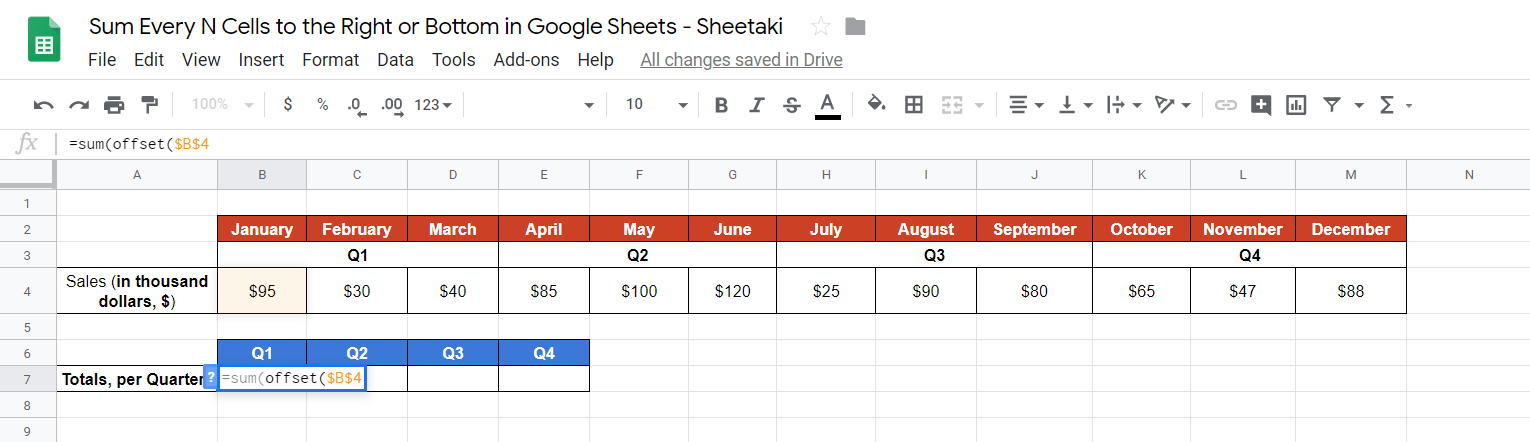
3. The next step is important – formulating our working formula. Remember that our goal is to sum every n cells to the right in Google Sheets. In this example, we need to sum up to the right on a per quarter basis which means sum every 3 cells to the right. That being said, a simple SUM formula won’t work. Therefore, we need to partner it with two other functions, OFFSET, and COLUMN. We will start our formula with the SUM function. Start off by entering the equal sign ‘=‘ to begin our function then enter ‘SUM‘ followed by an opening parenthesis ‘(‘.

4. So next is to use the OFFSET function. This function is useful especially when we are working with rows and columns where we want to sum every n number of cells horizontally or vertically. Once you’re written the OFFSET function, make sure you follow it by an opening parenthesis ‘(‘ as we always do for every function in Google Sheets.

Read More: How to Use OFFSET Function in Google Sheets.

5. Now, we will have to supply the attributes of the OFFSET function. We will be using the OFFSET function to shift every n cells to the right as we sum. Now to start off the OFFSET function, we will provide our first attribute which is cell_reference (or in order words the starting point). Hence click on the first data in our sales, which is $95 from the month of January. Make sure that you add the dollar ‘$‘ signs for the cell_reference like $B$4 as this means an ‘absolute’ or ‘constant’ value. When a cell is made absolute/constant, it never changes when we drag the cell across horizontally when we want to obtain the sum every n cells to the right.

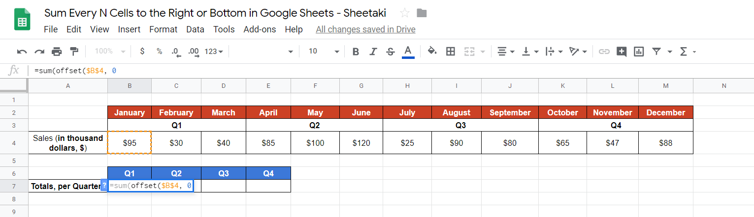
6. Good work! Next, since we do not want anything for the offset_rows attribute of OFFSET function, we will add “0” here instead. Why “0″ you may ask? It’s because we’re trying to sum towards the right which means we jump between columns and not rows. The offset_rows attribute will be crucial when we talk about how to sum every n cells to the bottom later in this guide. Hence, for now, we will be using offset_columns instead where we will utilize the COLUMN function in the next step.

7. Now the COLUMN function can be a tad bit difficult to understand for some, but it’s actually pretty simple! The COLUMN function basically returns the column number for any cell. In this part, we will be writing: (column()-column($B$4))*3. This formula is like the brains of this whole solution as it is responsible for making the sum every n columns to the right work. The attribute column() returns the column number, and in this case, it returns 2 at cell B7. The column($B$4) in the formula is also 2. Therefore, when we combine both of these, it will be (2-2)*3=0 in cell B7. 

8. Now to explain it to you in greater detail, if you were to just enter the formula =(column()-column($B$4))*3 here, hit Enter and then drag the cell towards the right and you should find that the subsequent cells will be followed by 0 (2-2)*3, 3 (3-2)*3, 6 (4-2)*3, and so on. This is the ‘jump’ factor. Meaning, 0 will later (once we finish the formula) be the first three cells from the cell_reference to be summed up, followed by 3 or otherwise known as the third cell from the cell_reference and it’s subsequent three cells to be summed up, and so on.

9. Now back to our formula, we will then add the other attributes for our OFFSET function which are the height and width with values of 1 and 3 respectively. The number 1 signifies that there is only one row to sum, while the number 3 decides the ‘n‘. Now, why did I decide on n to be 3? Well as aforementioned, we want to sum for every quarter where every quarter has three months. Hence, we sum every 3 cells to the right and which is why n is set to 3.

10. Close our OFFSET and SUM formulas with a close parenthesis ‘)‘ (as shown below)

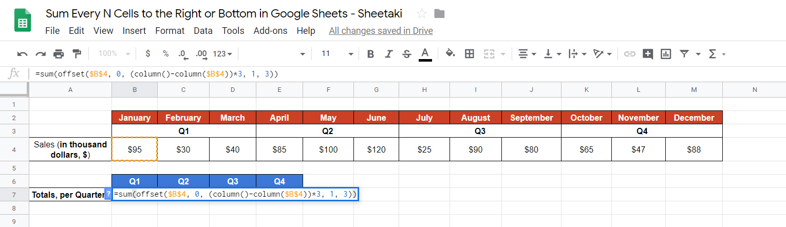
11. Hit the Enter key then drag the formula to the right. There you have it! As you can see for each quarter the value is output. For instance, Q1 is $165 ($95+$30+$40), Q2 is $305 ($85+$100+$120), Q3 is $195 ($25+$90+$80) and Q4 is $200 ($65+$47+$88).

In the end, your formula should look like this:

=sum(offset($B$4, 0, (column()-column())*3, 1, 3))

And that’s how you sum every n cells to the right in Google Sheets. Easy, right?

Feel free to make a copy of the example spreadsheets for the Sum-Right which we discussed above to try and see how it is done. Experiment with it and you will go through the above steps once again on your own using a different cell reference or different sets of data.

We’ll move on to the second example, which is, to sum every n cells to the bottom in Google Sheets. The steps are pretty much exactly the same as above only that we will be using the offset_rows attribute.

How do we do this? Easy peasy.

How to Sum Every N Cells to the Bottom in Google Sheets: 7 Steps

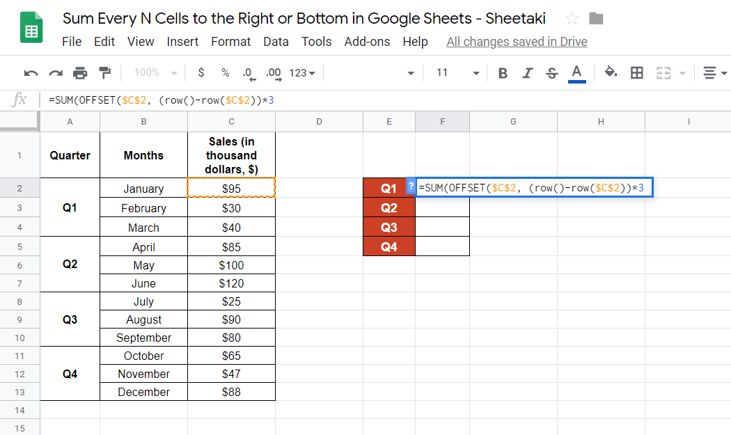
1. We will prepare our sales values using the same data as above. The only caveat is that whenever we want to sum every n cells to the bottom, which case we will need to write it vertically. Here’s what I mean:

2. Next, we will click on any cell to make it active. For this guide, I will select the cell E2.

3. Let’s start our formula with an equal sign ‘=‘ and the SUM function together with an opening parenthesis ‘(‘.

4. Same as in our example above, we will also use the OFFSET function, followed by our cell reference, which is C2. Don’t forget to add a dollar sign ‘$‘ to make this value absolute.

5. Next is to write this part in our working formula: $C$2,(row()-row($C$2))*3. We just modified the column function into a row. You can see how similar it is to what we did back in Step 7 above when trying to sum n cells to the right.

6. Then, we will supply the offset_columns, height, and width attributes by adding 0, 3, and 1.

7. Let’s now close our OFFSET and SUM formulas with a close parenthesis ‘)‘ (as shown below) then we hit Enter.

8. Then, we drag our formula down.

In the end, your formula should look like this:

=sum(offset($C$2, (row()-row($C$2))*3, 0, 3, 1))

Again, feel free to make a copy of the example spreadsheets for both (Sum-Right and Sum-Bottom) which we discussed above to try and see how it is done. The most important lesson is you should have fun doing it.

That’s pretty much it. Well done! 👏🏆

Let us know how it goes down below and we will try our best to reply to you and help you or even have a look at your finished work. Also while you’re at it, why not check out the other numerous Google Sheets formulas to create even more powerful formulas that can make your life much easier. 🙂

Get emails from us about Google Sheets.

Our goal this year is to create lots of rich, bite-sized tutorials for Google Sheets users like you. If you liked this one, you'll love what we are working on! Readers receive ✨ early access ✨ to new content.

Subscribe