How to Use UNARY_PERCENT Function in Google Sheets

The UNARY_PERCENT function in Google Sheets is useful if you want to interpret a number into a percentage value.

The UNARY_PERCENT does this simply by combining the syntax together with a number, or if the number is in the cell, you can just click the specific cell.

You may not find the UNARY_PERCENT function necessary, but inevitably it comes handy, especially when working on complex or large data spreadsheets.

Let’s take an example to understand this function better.

Say, for example, you are in charge of preparing a budget for your department. The management allocated $50,000 for your department’s needs, and you have to supply a budget report.

So how do we do that?

Simple. First, we identify our department’s necessities and arrange them according to priority. Then, we can use the UNARY_PERCENT function to convert the numbers into percentage values. Then, we will now multiply the percentage value with the said budget to arrive at a certain amount per need.

See how easy that is?

Another example that the UNARY_PERCENT function may be helpful is when we deal with financial and/or loan calculations using functions like PMT, IPMT, PPMT, and so on. We can have the UNARY_PERCENT nested in those formulas for you to arrive at a precise answer in an instant.

Let’s dive into real-business examples where we will deal with actual values and textual strings to appreciate the concept and how we can write our own UNARY_PERCENT function in Google Sheets to compute those data.

The Anatomy of the UNARY_PERCENT Function

So the syntax (or the way we write) the UNARY_PERCENT function is as follows:

=UNARY_PERCENT(percentage)

Let’s break this down to understand better what each of the terms means:

• = the equal sign is just how we start any function in Google Sheets.
• UNARY_PERCENT() is our UNARY_PERCENT function where it will return a PERCENTAGE value.
• PERCENTAGE is the value that we want to interpret as a percentage (e.g. 20, 40, 100, or a selected cell in a sheet that contains a number)

A Real Example of Using UNARY_PERCENT Function

Take a look at the example below to see how UNARY_PERCENT functions are used in Google Sheets.

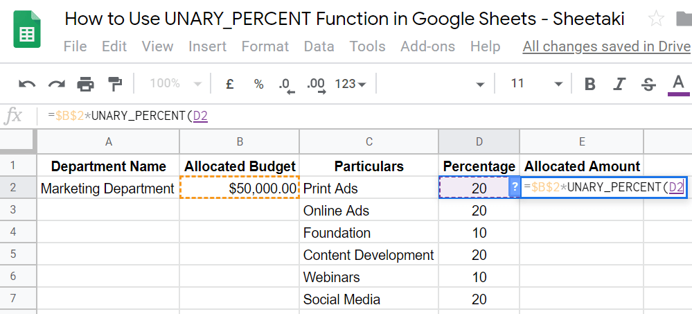
In the example above, the UNARY_PERCENT is used to convert the numbers in column D into percentage values. We then multiplied the allocated budget with the UNARY_PERCENT value to arrive at the allocated amount. Since our allocated budget of $50,000 is constant, we made use of the dollar ($) symbol to make it absolute.

=$B$2*unary_percent(D2)

Here’s what this example does:

• We have listed in column C as particulars all the marketing activities that our marketing department will take on. We also specified the percentage value for each activity, as seen in column D.
• Then, we have selected the cell E2 to make it an active cell. This is where we wrote our formula.
• We started our formula with an equal sign ‘=‘ followed by an opening parenthesis ‘(‘ and the cell B2.
• Since we wanted to make B2 absolute, we added a dollar sign ($) before the letter B, and another dollar sign before the number 2 ($B$2).
• Now, we multiply $B$2 with the percentage value. Since the percentage in column D are presented in numbers, we, therefore, need to transform them by using UNARY_PERCENT.
• Close the formula with a close parenthesis ‘)‘, then hit on the Enter key.
• Make sure your formula should look like this: =$B$2*unary_percent(D2), before dragging it down to E7.

Super easy, right?

You may make a copy of the spreadsheet using the link I have attached below:

Get emails from us about Google Sheets.

Our goal this year is to create lots of rich, bite-sized tutorials for Google Sheets users like you. If you liked this one, you'll love what we are working on! Readers receive ✨ early access ✨ to new content.

Subscribe