


This guide will explain how to use the WRAPROWS function in Google Sheets to form a new output.
When we want to wrap a provided row or column of values, we can easily do it using the WRAPROWS function in Google Sheets.
The rules for using the WRAPROWS function in Google Sheets are the following:
- The
WRAPROWSfunction is used to wrap the provided row or column of values into a row. - The wrap_count argument must be a whole number. When we input a value that is not a whole number, it will round down to the nearest whole number.
- If we leave the pad_with argument blank, the function automatically fills the extra cells with #N/A.
Google Sheets offer several built-in functions that allow us to easily perform tasks. Recently, they released multiple new functions that belong to the array category. For example, they released WRAPCOLS and WRAPROWS.
Previously, we had to wrap texts using the text wrapping tool or applying functions such as SEQUENCE and VLOOKUP. Now, we can now easily wrap values into rows or columns using a single function.
However, the new functions may not be fully rolled out yet to all users. If Google Sheets return a #NAME? error when you try to use the WRAPROWS function, it means the function is not yet available in your Sheets.
In this guide, we will provide a step-by-step tutorial on how to use the WRAPROWS function in Google Sheets. Additionally, we will explore the syntax and a real example of using the function.
Great! Let’s dive right in.
The Anatomy of the WRAPROWS Function
The syntax or the way we write the WRAPROWS function is as follows:
=WRAPROWS(range,wrap_count,[pad_with])
- = the equal sign is how we begin any function in Google Sheets.
- WRAPROWS() refers to our
WRAPROWSfunction. This function is used to transform the provided row or column of cells by rows. - range is a required argument. This refers to an array or range we want to wrap. Additionally, this can be a single column or row.
- wrap_count is another required argument. This refers to a number representing the maximum number of cells for each row in the returning result or output.
- pad_with is an optional argument. This allows the function to replace the extra blank cells with a given value. By default, the function inputs #N/A in the extra blank cells.
A Real Example of Using WRAPROWS Function in Google Sheets
Let’s say we have a data set consisting of the quarterly sales in one year. But, the values for the months under each quarter are simply listed in one long column.
Our initial data set would look like this:

In the spreadsheet above, we can see that the list is divided by the quarter such as Quarter 1, Quarter 2, Quarter 3, and Quarter 4. In each quarter, there are three values listed which are the total sales for each month in that quarter.
We want to create multiple rows to display the monthly sales of each quarter and the labels at the leftmost cell to be included in each row.
We can easily perform this by using the following formula:
=WRAPROWS(B3:B18,4)
The first argument of the function is the location of the list of values we want to wrap. The second argument indicates how many cells we need for each row.
Additionally, we can utilize the optional pad_with argument to input a specific value or text in the extra blank cells.
For example, we can input 5 as our wrap_count which would give us extra cells. Then, we can type the “unavailable” at the end of our formula to be displayed in the blank cells.

Since there are 3 months in each quarter plus a cell for the label, we need a total of 4 cells. If we place a value that is not a whole number, the function will automatically round down to the nearest integer.
For instance, we input the value 3.5 as the wrap_count argument. The function will round it down to 3 and return 3 cells for each row.

Thus, our final data set with wrap_count 4 would look like this:

You can make your own copy of the spreadsheet above using the link below.
Amazing! Now we can dive into the steps of using the WRAPROWS function in Google Sheets.
How to Use WRAPROWS Function in Google Sheets
1. First, we will select an empty cell where we can input our WRAPROWS formula. Make certain that there is enough space to display the output you want to return.

2. We will input “=WRAPROWS(“ to start our formula.

3. Now we need to select the group of cells containing the values we want to wrap. In this case, we will select B3:B17.

4. Next, we will input how many cells we want in each row. In this case, we need 4 cells. Then, the formula would be “=WRAPROWS(B2:B17,4)”.

5. Additionally, we can use an optional argument to input a value for empty cells. In this case, we can type “unavailable” to replace the blank cells. Our formula will become “=WRAPROWS(B2:B17,4,”unavailable”)”.
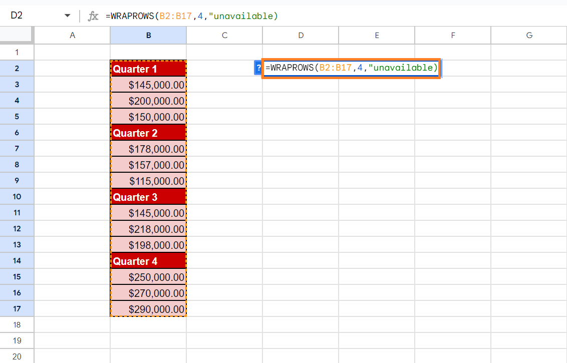
6. Lastly, press the Enter key to return the results.
And tada! We have successfully used the WRAPROWS function in Google Sheets.
You can apply this guide whenever you need to transform a row or column into multiple rows. You can now use the WRAPROWS function and the various other Google Sheets formulas available to create great worksheets that work for you.
FAQs:
1. What is the difference between WRAPROWS and WRAPCOLS functions?
The WRAPROWS function wraps the provided row or column by rows. On the other hand, the WRAPCOLS function wraps the provided list of values by column.
2. Are there any alternative methods or functions to achieve text wrapping in Google Sheets?
Yes, Google Sheets provides a built-in Wrap option in the Text wrapping menu that allows you to wrap text within a single cell. You can also use the ALT+ENTER keyboard shortcut to manually add line breaks within a cell to achieve text wrapping.
3. Can I use the WRAPROWS function in conjunction with other functions in Google Sheets?
Yes, you can use the WRAPROWS function in conjunction with other functions in Google Sheets to create more complex formulas and calculations.
That’s pretty much it! Make sure to subscribe to our newsletter to be the first to know about the latest guides and tutorials from us.


