How to Add and Edit a Trendline in Google Sheets

Adding a trendline in Google Sheets lets you show the general trend of datasets in your chart.

Sometimes, charts may not show enough information about your data. So, you may miss important insights, such as event patterns over time.

Fortunately, Google Sheets allows you to add trendlines to your charts. A trendline is a line that illustrates the movement or trend of data points in a chart. Whether you are using a line, bar, scatter, or column chart, consider adding a trendline to improve how it presents your data.

There are various types of trendlines available in Google Sheets. Depending on what you need, you can choose among trendline types such as Linear, Exponential, Polynomial, Moving Average, and many others.

It’s quite easy to add a trendline. In this tutorial, we will demonstrate how to do it and show how you can edit it to suit your needs.

Let’s get started!

A Real Example of a Trendline in Google Sheets

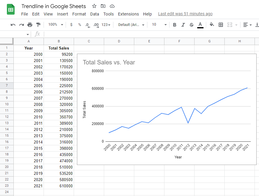
Here is a spreadsheet that shows a company’s total sales over the past two decades.

The raw data above would be more meaningful if it were illustrated using a line chart. This will show us the whole picture of sales increases and decreases over time, as shown in the example below:

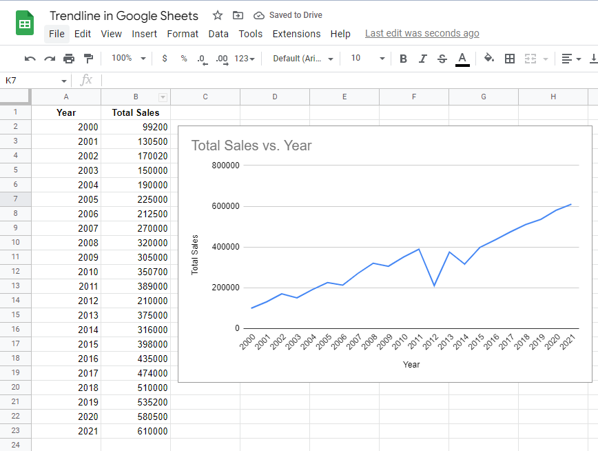
While the line chart already gives us a general idea of the total sales per year, it would be better if we could add a trendline to easily identify the overall direction of the data.

From a plain line chart like the one earlier, you can easily convert it into something like this:

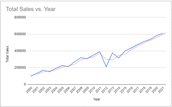
Notice the red line in the chart above. This is a type of trendline called Moving Average. Trendlines like this one can give you additional information about the overall behavior of your data.

So, how can you add a trendline to your chart in Google Sheets? Let’s find out in the next section.

How to Add a Trendline in Google Sheets

Since a trendline is part of a chart, obviously, you need to create a chart first in your spreadsheet before you can add one. Click the link below to make a copy of our own spreadsheet, so that you can practice on it.

1. As you can see, the example spreadsheet already contains a line chart beside the dataset. Our objective for this activity is to add a Moving Average trendline to smoothen out the data.
   
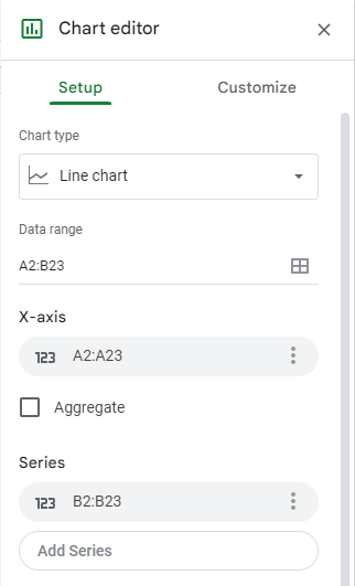
2. Let’s start by displaying the Chart editor panel. To do so, double-click on the line chart. You’ll notice that a panel similar to the image below, will appear on your screen.
   
   
3. Next, navigate to the Customize tab of the Chart editor.
   
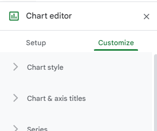
4. From the Customize tab, proceed to the Series section. Click on it to display the controls under it.
   
   
5. This time, scroll down until the end of the Series section. There, you’ll find the Trendline checkbox. Check it to add a default trendline to the line chart.
   
   
   
   Upon doing all the steps above, the line chart should now look like this:

Ticking the trendline checkbox adds a default trendline to your chart. In our case above, a Linear trendline is added with a light blue color. This can be confusing as the main line also has a blue color. But don’t worry, we can customize this trendline and give it a different color and look. You’ll learn how to do this in the next section.

Editing a Trendline in Google Sheets

After adding a trendline to your chart, you can customize its appearance to put more emphasis on it. Here’s how to do so:

1. First, ensure that the Chart editor panel is displayed on your screen. You can do it by simply double-clicking the line chart.
2. Afterward, navigate to the Customize tab and head over to the Series section.
3. You’ll notice the set of controls below the Trendline checkbox. Use these tools to edit the appearance of the trendline in your chart.
   
   
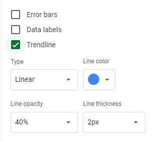
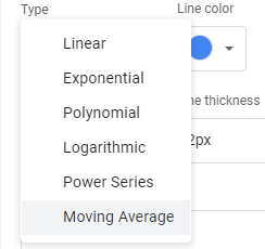
4. You can change the type of trendline by clicking the Type drop-down button. Doing so will display the list of trendlines supported by Google Sheets. From the list, click the type of trendline you want to apply. For the purposes of this guide, let’s select Moving Average.
   
   
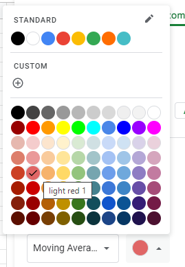
5. The next thing you need to do is change the trendline’s color so that you can easily distinguish it from the main line. Click the Line color drop-down button and then choose light red. Refer to the image below to apply the exact color.
   
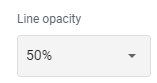
6. Now that we’re done with the type and color, let’s proceed with the opacity and line thickness. The Line opacity field determines how transparent the line is. In our case, let’s set it to 50 percent, as shown in the image below.
   
   
   
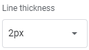
   For the line thickness, let’s set it to 2px:
   
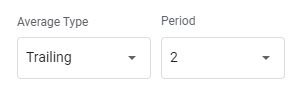
7. Besides color and thickness, there are additional fields that can be used for overriding the appearance of your trendline. These fields vary depending on the type of trendline you have selected. In the case of the Moving Average trendline, you can modify the average type and period fields using their respective fields:
   
   
8. Once you’re done editing the trendline, the line chart should now look like this:
   
   

That’s about it! You just learned how to add and edit a trendline in Google Sheets. Remember to use this feature if you need to illustrate the overall trend of data in your chart.

Browse our other articles on Google Sheets if you’re interested in learning more.

Sign up for our newsletter to learn more about other Google sheets essentials.

Get emails from us about Google Sheets.

Our goal this year is to create lots of rich, bite-sized tutorials for Google Sheets users like you. If you liked this one, you'd love what we are working on! Readers receive ✨ early access ✨ to new content.

Subscribe