ForssThe FV function in Excel is useful when you need to use the compound interest formula to determine the future value of an investment.
The formula can be used for either periodic payments or a single lump-sum payment.
The rules for using the FV function in Excel are as follows:
- The function requires three arguments: the interest rate per period, the total number of payment periods, and the payment made in each period.
- The user has the choice to fill in two optional arguments: the investment’s present value, and whether payments are due at the beginning or end of the period.
- The function then outputs a number that refers to the future value of an investment given a constant interest rate.
Compound interest refers to the interest gained from both the initial principal amount and any prior interest added to that amount. In short, compound interest is partly interest earned on prior interest.
Let’s take a look at a quick example where we can use a compound interest formula.
Suppose you’ve placed $100 of savings in an account that pays 2% annual interest. After the first year, you will have an additional $2 of interest. As a result of compound interest, you will earn $2.04 or 2% of 102 in the second year, slightly more than the original payout of $2.
Given a fixed interest rate, how can we compute the value of our investment in 10 years?
With the FV function, it becomes quite easy to calculate the future value of an investment with a fixed interest rate.
Because we now know when to use the FV function, let’s take a look at what arguments are needed for this function.
The Anatomy of the FV Function
The syntax of the FV function is as follows:
= FV(rate, nper, pmt, [pv], [type])
Let’s dissect this formula and understand what each of these terms means:
- The equal sign ‘=’ is how we indicate the start of any formula in Excel.
- FV() is our
FVfunction. This financial function computes for the future value of a given investment. - rate refers to the interest rate per period
- nper is the total number of payment periods in the lifetime of the investment
- pmt is the payment made in each period.
- pv is the present value or the lump sum amount.
- type is the argument that indicates when payments are due. For instance, a type of 1 indicates that payments are due at the beginning of the period. If the type is 0, then payments are due at the end of the period.
A Real Example of Using the FV function to get the Compound Interest in Excel
Let’s take a look at a real example of the FV function being used in an Excel spreadsheet to compute for compound interest.
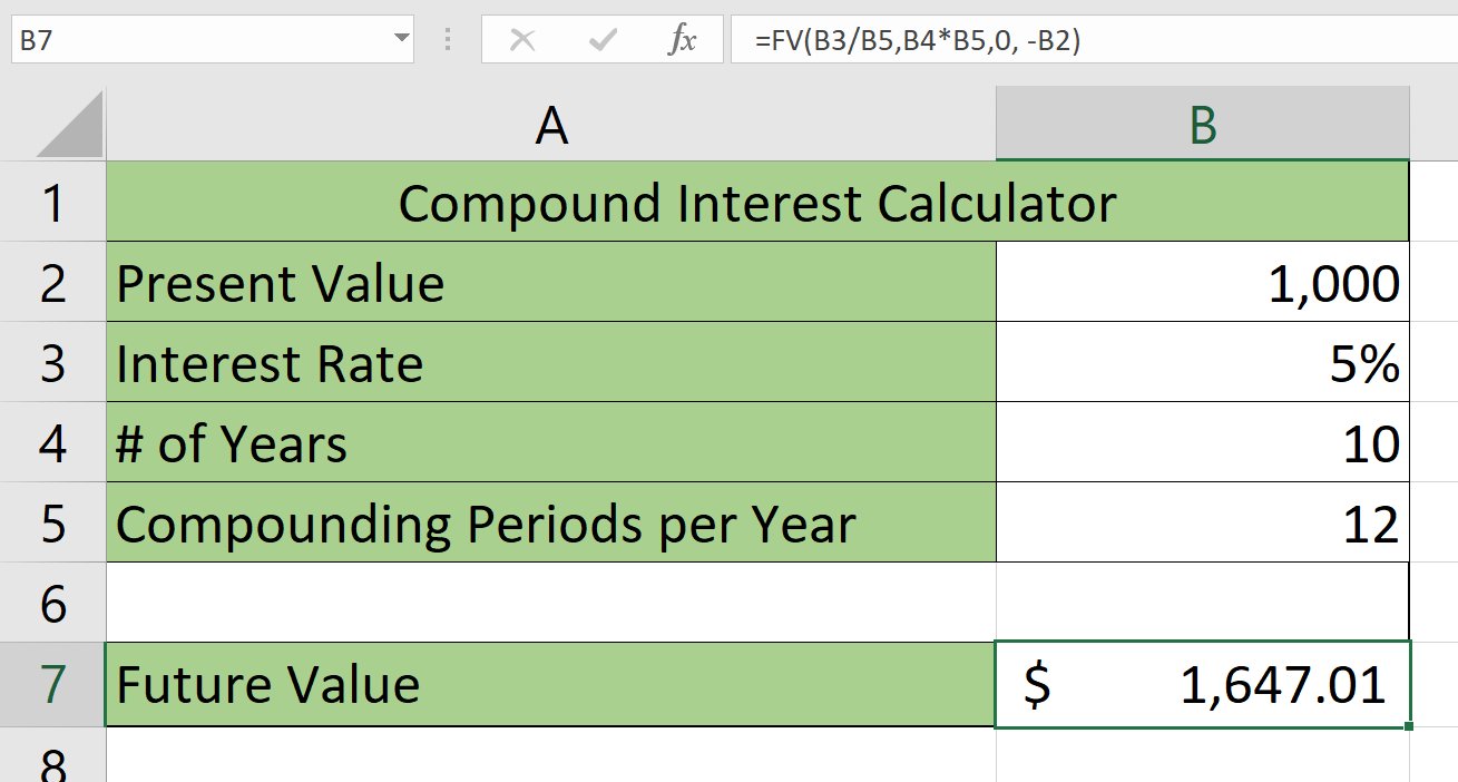
In the example below, we’ve set up a compound interest calculator that makes it easier to solve for the future value of your investment.

To get the result in cell B2, we just need to use the following formula:
=FV(B3/B5,B4*B5,0, -B2)
You can make your own copy of the spreadsheet above using the link attached below.
If you’re ready to try out the FV function in Excel, let’s begin writing it ourselves!
How to Use Compound Interest Formula in Excel
This section will guide you through each step needed to start using FV in Excel. You’ll learn how we can use this function to solve compound interest for an investment.
Follow these steps to start using the FV function:
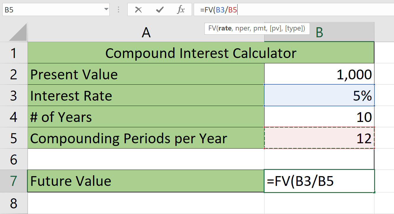
- First, set up the compound interest calculator by adding the necessary template. We’ll be needing four cells for user input.

- Next, you can start the compound interest formula by adding the string ‘=FV(‘ to start the
FVformula.

- For the first argument, we’ll need to divide our interest rate by the number of compounding periods per year. In this example, we will divide our interest rate of 5% by 12.

- Our second argument requires the number of compounding periods to compute for. We can calculate this by multiplying the number of years in cell B4 with the number of compounding periods in a year specified in B5.

- We leave our third argument blank since we’ll be using a lump sum payment. We’ll then specify our present value in the fourth optional argument. Hit the Enter key to evaluate the function. In our example, we’ve accrued $647.01 in interest after 10 years.

- Users of this sheet can quickly change each variable to solve for different types of investments.

This step-by-step guide should be all you need to start solving for compound interest in Excel. In addition, our guide shows how easy it is to use the FV function to track how much an investment grows over time given a fixed interest rate.
The FV function is just one example of a financial function you can use in Excel. With so many other Excel functions available, you can surely find one that suits your use case.
Are you interested in learning more about what Excel can do? Subscribe to our newsletter to find out about the latest Excel guides and tutorials from us.


