This guide will explain how to use the bicubic interpolation in Excel.
Table of Contents
Bicubic interpolation in mathematics is a method used to approximate values between discrete data points by fitting a bicubic polynomial to a set of neighboring data points.
Moreover, this technique is commonly applied in numerical analysis, computer graphics, and image processing.
Since Excel does not have a built-in bicubic interpolation function, we will define our custom function to calculate the interpolated value f (x,y) at the desired (x, y) coordinates.
In this guide, we will provide a step-by-step tutorial on how to do bicubic interpolation in Excel.
Additionally, we will explore the syntax of the functions we will use and a real example of performing bicubic interpolation.
Great! Let’s dive right in.
A Real Example of Doing Bicubic Interpolation in Excel
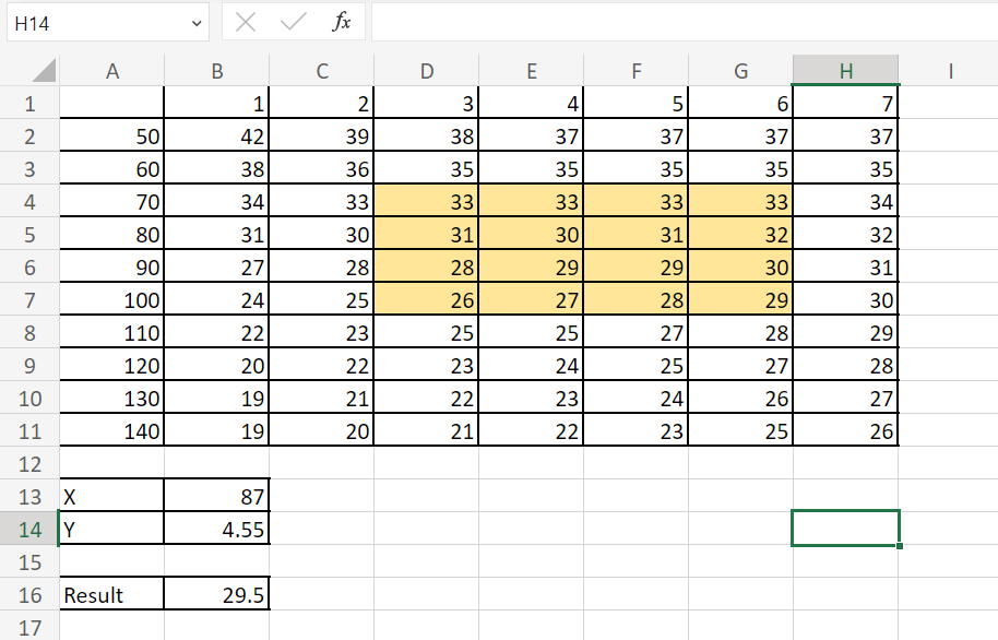
Let’s say we have a grid of points, and we need to find the values somewhere between the points. For example, our initial data set would look like this:

To perform bicubic interpolation, you need to set up a 4×4 grid of data points centered around the interpolation point (x=87, y=4.55).
To create a 4×4 grid, we will populate the grid with values from our dataset corresponding to the nearest data points. Moreover, make sure we have 16 data points available.
Then, we will calculate the coefficients of the bicubic polynomial based on these 16 data points. However, we would typically need to perform a series of calculations and solve a system of linear equations based on the data set.
Since Excel does not have a built-in bicubic interpolation function, we will add the functionality using VBA code that calculates the coefficients for bicubic interpolation based on a given dataset and then performs bicubic interpolation at a specified (x, y) coordinate.
You can access this Google Drive link to see the VBA code used in our worksheet.
Once we’ve successfully added the custom code as a new module in our worksheet, we now have access to the custom BicubicCoefficents and BicubicInterpolation functions.
We can use the BicubicCoefficients to calculate the coefficients based on your 4×4 grid of data points and the BicubicInterpolation to estimate values at specific (x, y) coordinates within the grid, passing the calculated coefficients as an argument.
In this example, we want to perform bicubic interpolation to estimate the value at point (x=87, y=4.55).
To calculate the coefficients, we will use the formula below:
=BicubicCoefficients(D4:G7)

Once we have the coefficients, we can now perform the bicubic interpolation.
We can apply the formula:
=BicubicInterpolation(B13,B14,$D$4:$G$7,$J$2:$M$5)
We are using absolute references ($) in our formula to lock the column and cell references. Thus, this will ensure that copying the formula to another cell does not change the formula references.

Our final data set would look like this:
You can make your own copy of the spreadsheet above using the link below.
Amazing! Now, we can dive into the steps of doing bicubic interpolation in Excel.
How to Do Bicubic Interpolation in Excel
1. First, we need to have access to the Developer tab. If you do not see the Developer tab in the ribbon, we have to enable it first through the Excel options dialog box. To do this, we will click on the Options button in the File tab to view the dialog box seen below.
Next, we will head to the Customize Ribbon options and check the Developer option under the list of main tabs to display. Lastly, click OK to apply these changes.

2. Secondly, we can head over to the Developer tab and select the Visual Basic option.

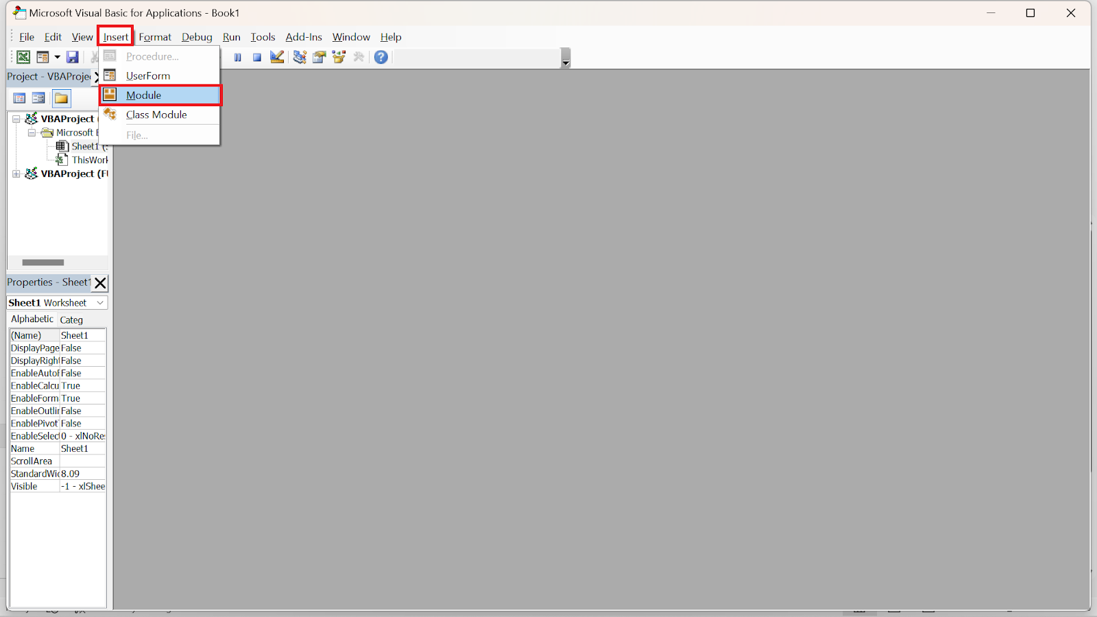
3. Then, a Visual Basic editor will appear in a new window. Next, we will go to the Insert tab and click Module in the dropdown menu.
4. In the window, we can paste our VBA code. To do this, we can right-click and select Paste. Otherwise, we can also simply press Ctrl + V. Lastly, we will click the Save icon and close the application.

5. Afterward, we need to save our workbook as macro-enabled. In the Save as window, we can choose Excel Macro-Enabled Workbook in the pop-up menu. Lastly, we will click Save to apply the changes.

6. Next, we will head back to our worksheet and prepare our data set. Since we already have our 4×4 grid, we will now calculate the coefficient using the BicubicCoefficients function we got from our VBA code.
Hnce, our formula to get the 4×4 grid point coefficients would be “=BicubicCoefficients(D4:G7)”.

7. We will press the Enter key to return the results. The function will output an array of the coefficients.

8. Now that we have our coefficient, we can perform the bicubic interpolation. To begin, we will type in the function name “=BicubicInterpolation(“.

9. Then, we will select the cells containing the x and y coordinates where we want to interpolate. Thus, our formula would become “=BicubicInterpolation(B13,B14”.
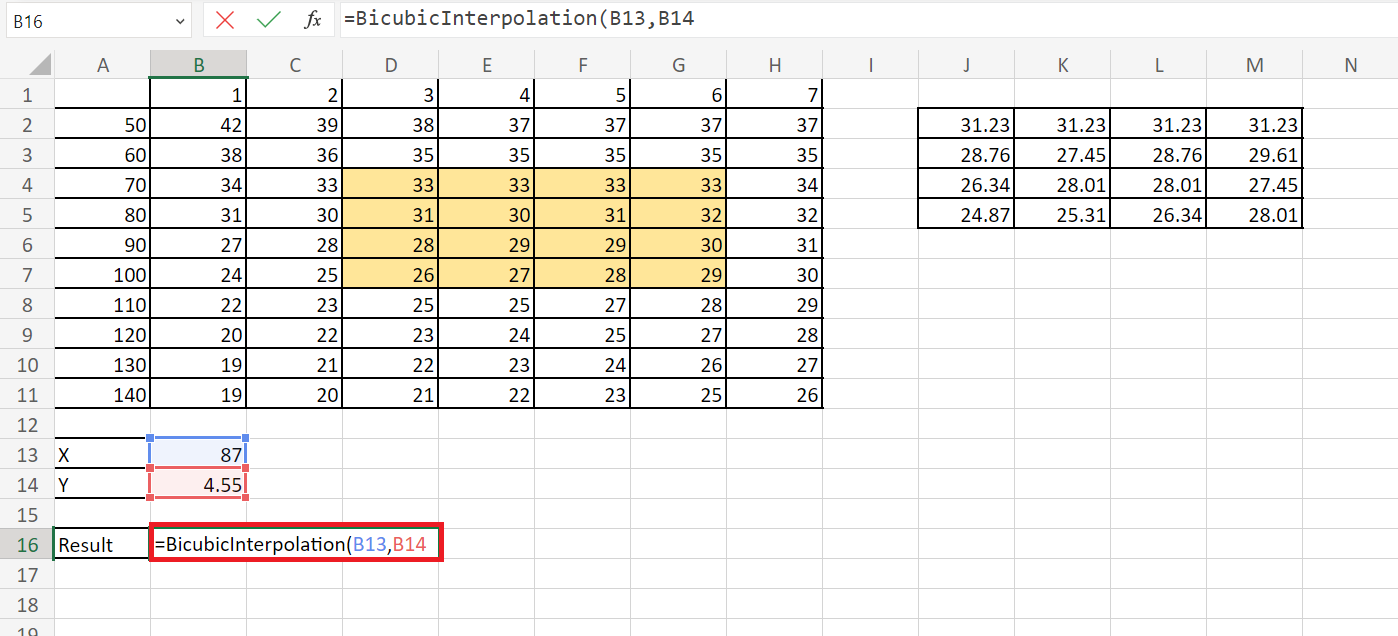
10. Next, we will select the range of our 4×4 grid of neighboring data points. Then, our formula would become “=BicubicInterpolation(B13,B14,$D$4:$G$7”.
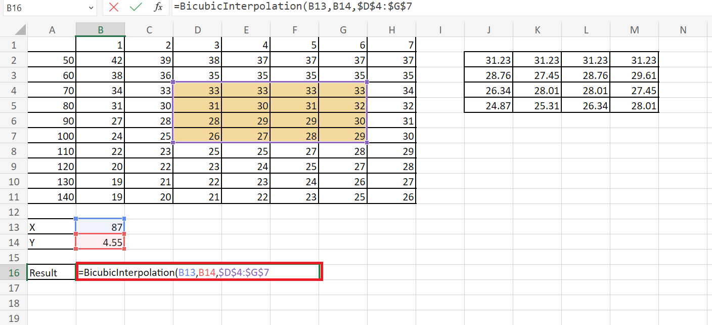
11. Lastly, we will select the range containing the coefficients. Our final formula would be “=BicubicInterpolation(B13,B14,$D$4:$G$7,$J$2:$M$5)”.

12. Lastly, we will press the Enter key to return the results.

And tada! We have successfully done bicubic interpolation in Excel.
You can apply this guide whenever you need to estimate values between discrete data points. You can now use the various other Microsoft Excel formulas to create great worksheets that work for you.
FAQ:
1. What are other interpolations I can perform in Excel?
You can perform linear interpolation in Excel, which helps estimate values based on two data points. If you have three variables like x, y, and z, where x and y are independent variables, and z is dependent on both, you can also do bilinear interpolation.
That’s pretty much it! Make sure to subscribe to our newsletter to be the first to know about the latest guides and tutorials from us.