


This guide will discuss how to use SUBTOTAL with SUMIF in Excel.
The rules for using the SUMIF function in Excel are the following:
- If sum_range is left blank or omitted, the function will calculate the sum of the same range as the condition.
- When we match strings longer than 255 characters with the function, it will return a #VALUE! error.
- Unless the criteria inputted is a numeric value, any text, logical values, and mathematical symbols inputted in the criteria argument must be enclosed with double quotation marks.
Excel can be used for many different tasks. Since it contains multiple built-in functions and tools, it makes calculations simple and easy. Additionally, we can manipulate and filter data easily.
However, filtering data cause some issues when we want to perform certain calculations on those data values. For example, we want to calculate the sum of specific cells from a filtered data set that meets our given criteria.
But, the function usually includes all the values filtered or hidden in the calculation. Thus, we cannot obtain the correct result we want from the function.
Instead of using a function alone, we can pair it with other functions to help perform the task we want to do. In this case, we want to calculate the sum of specific cells that meet our condition. But, the values are filtered from a larger data set.
Let’s take a sample scenario wherein we need to use SUBTOTAL with SUMIF in Excel.
Suppose you are a teacher who wants to calculate the sum of the scores of specific students in one class. Since your record contains a mixture of different classes, you have to filter your data set only to display the specific class you want to calculate the sum of scores.
Afterward, you can apply a combined formula of SUBTOTAL, SUMIF, and other functions to perform the calculator correctly.
Before we dive into a real example, let’s explain the syntax of the SUMIF function.
The Anatomy of the SUMIF Function
The syntax or the way we write the SUMIF function is as follows:
=SUMIF(range, criteria, [sum_range])
Let’s take apart this formula and understand what each term means:
- = the equal sign is how we can activate any function in Excel.
- SUMIF() refers to our
SUMIFfunction. And this function is used to add the cells specified by given criteria or conditions. - range is a required argument. And this refers to the range of cells we want to calculate the sum or be evaluated.
- criteria is another required argument. So it refers to the condition we input which is in the form of a number, expression, or text string that will decide which cells will be added.
- sum_range is an optional argument. And it refers to the actual cells to sum. If left blank, the cells in range will be used.
A Real Example of Using SUBTOTAL with SUMIF in Excel
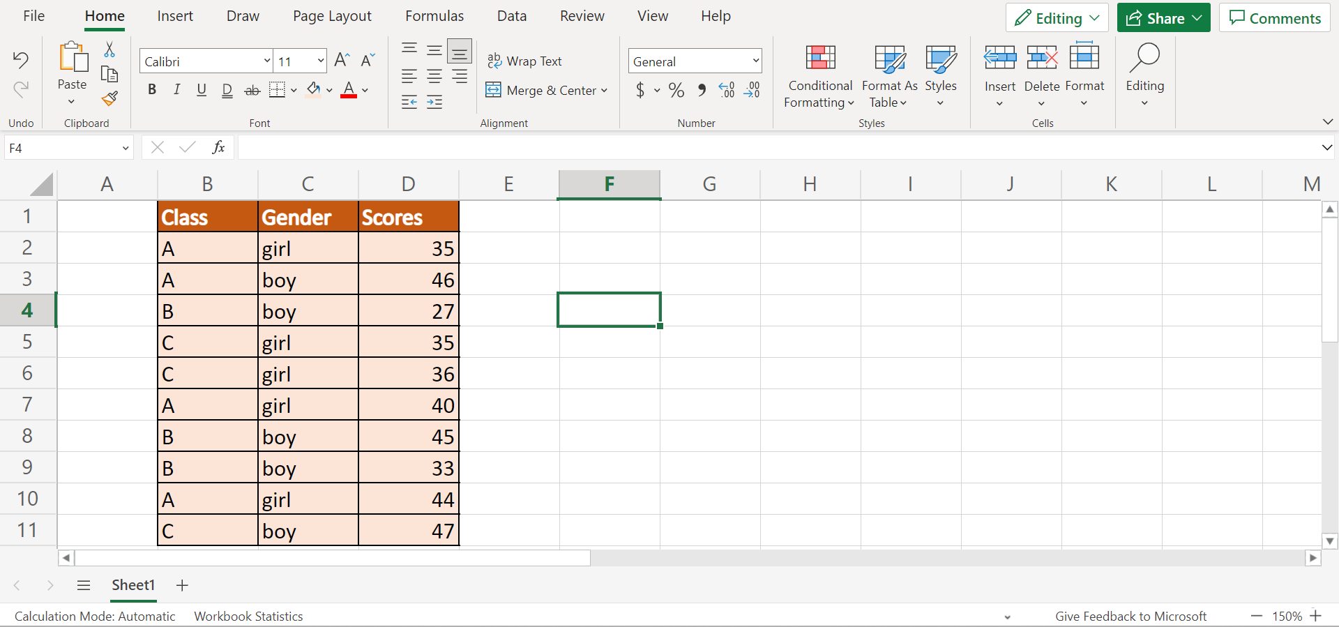
Let’s say we have a data set containing the different classes of the students, the gender of the students, and the score of each student. So our initial data set would look like this:
For instance, we want to calculate the sum of the scores of the girls within class C. Since the original data set contains all three different classes, we need to filter our data.
Firstly, we will filter our data set using the filter tool in the data tab. Once we only have the rows of class C displayed, we can proceed to our calculation. Essentially, we will combine functions to create a formula that will correctly return the sum of the scores.
So the SUBTOTAL function returns the subtotal of a list or database. Then, the SUMIF function calculates the sum of cells that meet the given criteria.
But, only using these two functions is not enough since we have a filtered data set. If we only use this formula, we will get a sum of the scores based on the entire data set instead of the filtered values.
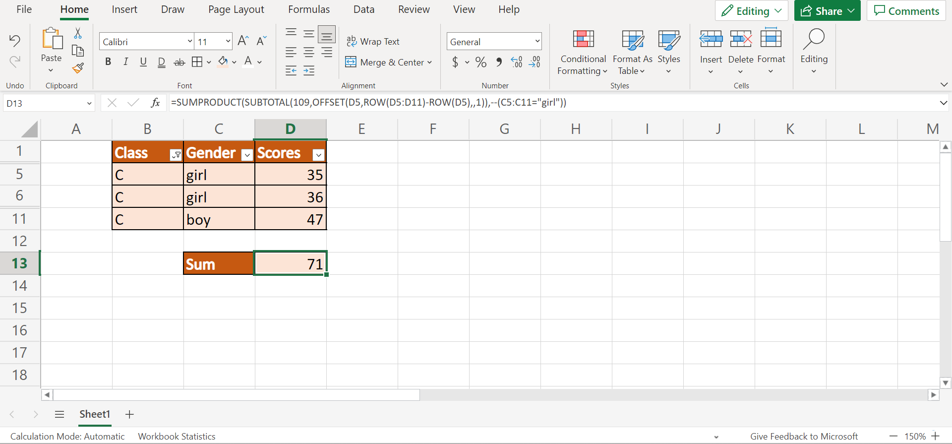
With the help of the SUMPRODUCT function, the formula will correctly filter the values and only return the sum of scores based on the filtered values. So our final data set would look like this:
You can make your own copy of the spreadsheet above using the link attached below.
Amazing! Now we can move on to the steps on how to use SUBTOTAL with SUMIF in Excel.
How to Use SUBTOTAL with SUMIF in Excel
In this section, we will explain the step-by-step process of how to use SUBTOTAL with SUMIF in Excel. Furthermore, each step contains pictures and detailed instructions to guide you along the way.
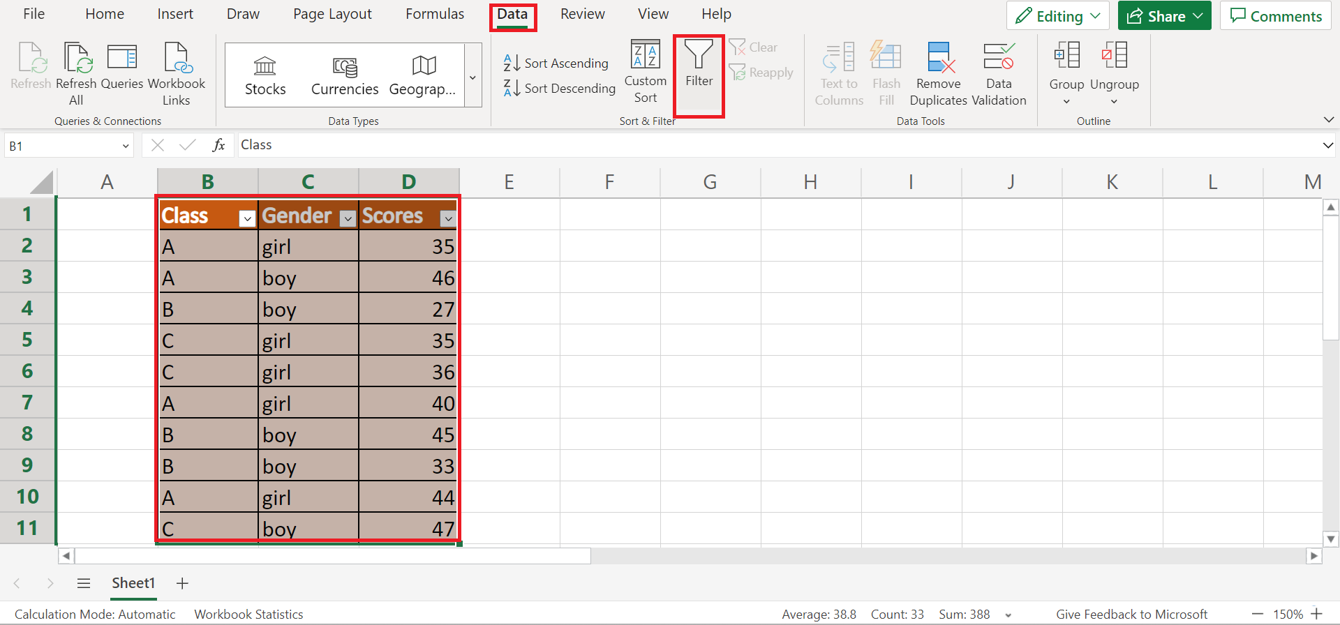
1. Firstly, we need to filter the data set. To do this, we must select the entire data set and go to the Data tab. Next, we will click the Filter icon in the Sort & Filter group.
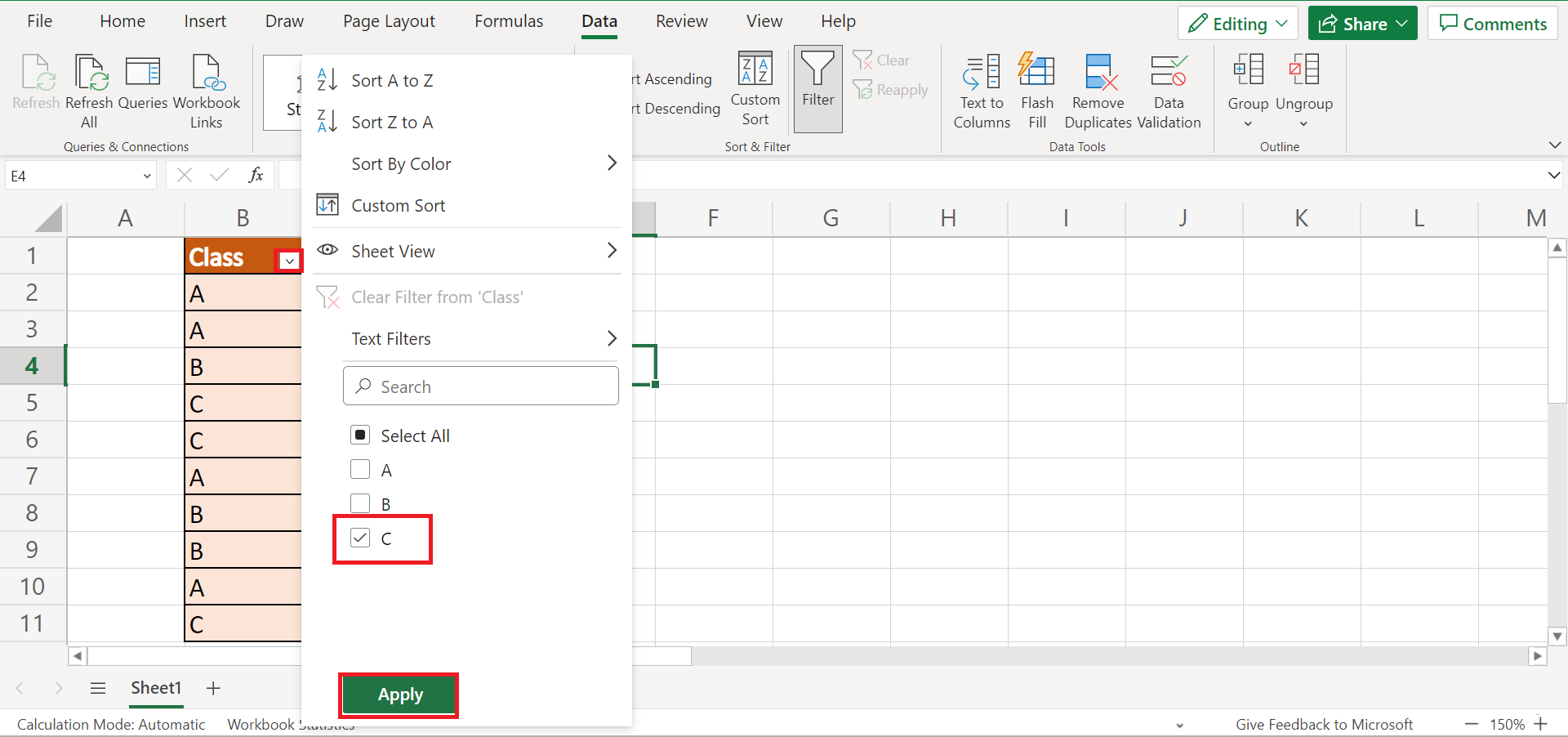
2. Secondly, we will display the specific cells we want. To do this, we will click the dropdown arrow beside the Class column. In the opened menu, we will check the box for C since we only want the rows from class C to be shown. Lastly, we will click Apply to filter the data set.
3. Then, we can proceed to calculate the sum of the scores of the cells that meet our criteria. In this case, we want to get the sum of the scores of the girls within class C. So we will type in the formula “=SUMPRODUCT(SUBTOTAL(109,OFFSET(D5,ROW(D5:D11)-ROW(D5),,1)),–(C5:C11=”girl”))”. Then, we will press the Enter key to return the result.

4. And tada! We have successfully used SUBTOTAL with SUMIF in Excel.
And that’s pretty much it! We have explained how to use SUBTOTAL with SUMIF in Excel. Whenever you need to calculate the sum of specific cells in a filtered data set, you can apply this guide to get the results correctly.
Are you interested in learning more about what Excel can do? You can now use the SUMIF function and the various other Microsoft Excel formulas available to create great worksheets that work for you. Make sure to subscribe to our newsletter to be the first to know about the latest guides and tutorials from us.


1 comment
Thank you so much. Your formula has been a great help to me