


This guide will explain how to do conditional formatting for blank cells in Excel using two simple methods.
Excel contains many tools and functions that we can use for various situations and purposes. And one of the most useful features Excel has is the conditional formatting feature. So conditional formatting allows us to highlight cells with a specific color depending on the rule or criteria we set.
Although conditional formatting has several rules or criteria we can choose from, we will focus on how to do conditional formatting for blank cells in Excel.
So one of the ways to perform this is by using the conditional formatting tool immediately. And another method is by using the ISBLANK function in Excel.
Furthermore, we need to understand that our definition of a blank cell may differ from how Excel defines a blank cell. Excel does not differentiate between a blank cell and a zero value.
For instance, we created conditional formatting to highlight cells containing values less than 10. So Excel would also highlight blank cells because 0 is less than 10, and Excel considers blank cells equal to the zero value.
Let’s take another example wherein we would need to perform conditional formatting for blank cells in Excel.
Suppose you are creating a sales report from the different store branch and their quarterly earnings. But, some of the stores have incomplete data. Thus, you ended up having blank cells in your data set. Before submitting the report, you wanted to highlight the blank cells to make them easier to spot.
And this is where you can utilize the conditional formatting tool or the ISBLANK function.
Great! Before we move on to a real example of doing conditional formatting for blank cells, let’s first learn how to write the ISBLANK function.
The Anatomy of the ISBLANK Function
The syntax or the way we write the ISBLANK function is as follows:
=ISBLANK(value)
Let’s take apart this formula and understand what each term means:
- = the equal sign is how we start any function in Excel.
- ISBLANK() is our
ISBLANKfunction. And this function will check whether the selected cell is an empty cell and will return a true or false value. - value is the only required argument for this function. And this refers to the cell reference we want to check whether it’s a blank cell or not.
And that’s it! Now we can discuss a real example of performing conditional formatting for blank cells in Excel.
A Real Example of Doing Conditional Formatting for Blank Cells in Excel
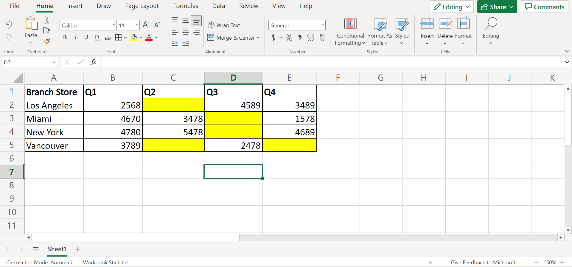
Let’s say we have a sales report containing some blank cells. And we want to highlight the blank cells to ensure that they can be easily spotted by someone viewing the report. So this is how our initial data set would look like this:

Then, we can utilize two methods to perform conditional formatting. Firstly, we can use the conditional formatting features in Excel, specifically the New Rules feature.
Secondly, we can use a formula to perform conditional formatting for blank cells using the ISBLANK function. And the ISBLANK function identifies only truly blank or empty cells meaning cells containing absolutely no spaces, no empty strings, no returns, no tabs, nothing.
Finally, our final output would look like this after doing conditional formatting for blank cells:
You can make your own copy of the spreadsheet above using the link attached below.
Awesome! Now we can learn the steps or process of how to do conditional formatting for blank cells in Excel using the two simple methods discussed above.
How to Do Conditional Formatting for Blank Cells in Excel
In this section, we will explain the step-by-step process of how to do conditional formatting for blank cells in Excel using two simple and efficient methods. Furthermore, each step will contain pictures and detailed instructions for you to easily follow.
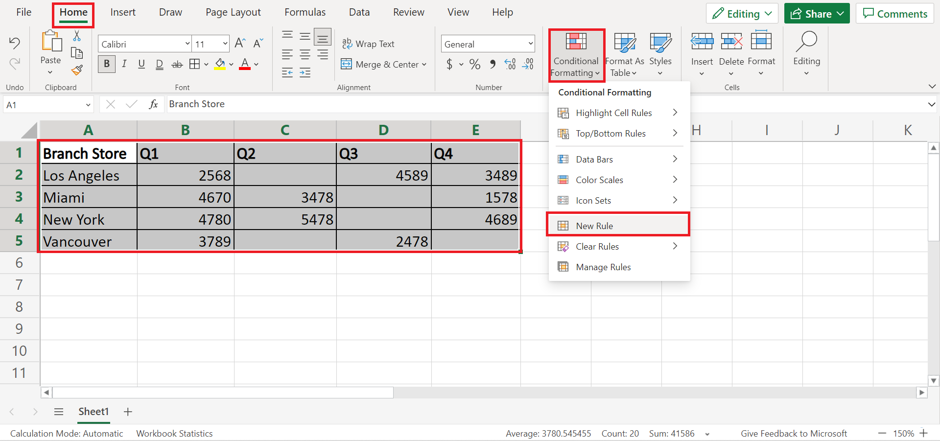
1. Firstly, we need to select the data set containing the blank cells. In this case, we will select A1:E5. Then, go to the Home tab and select Conditional Formatting. Next, click New Rule in the dropdown menu.
2. Secondly, the Conditional Formatting window will appear on the right side. In this window, select Highlight cells with under Rule Type. Next, choose Blanks in the Cell value dropdown menu.
Furthermore, we can customize the formatting of the blank cells under the Format with. In this case, we will highlight the cells in yellow. Lastly, click Done to apply the conditional formatting.

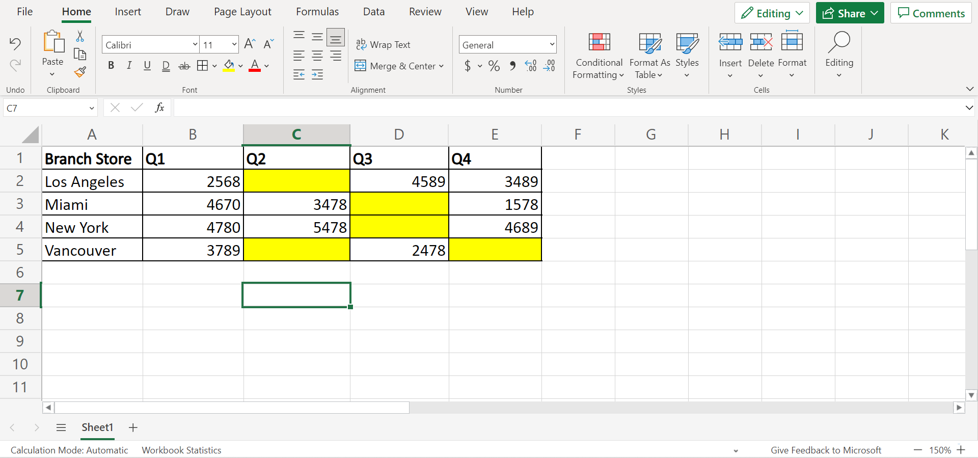
3. And tada! We have successfully formatted the blank cells to be highlighted in yellow.
4. Another method we can use is the ISBLANK function. To use this function, we need to go to the Home tab and select Conditional Formatting. Then, we will click New Rule in the dropdown menu.

5. Once the Conditional Formatting window opens, we must select Formula in the Rule Type dropdown menu. Then, we will input the formula in the space below that. In this case, our entire formula would be “=ISBLANK(B2)”.
Also, we can change the format to whatever color and style we want. In this case, we will choose yellow. Lastly, press Done to apply the conditional formatting.

6. And tada! We have successfully done conditional formatting for blank cells in Excel using two methods.
And that’s pretty much it! We have discussed thoroughly how to do conditional formatting for blank cells in Excel using two simple and easy methods. And now, you can apply any of these methods whenever you need to format blank cells in Excel.
Are you interested in learning more about what Excel can do? You can now use the ISBLANK function and the various other Microsoft Excel formulas available to create great worksheets that work for you. Make sure to subscribe to our newsletter to be the first to know about the latest guides and tutorials from us.


