This guide will explain how you can add a calculated field to a Pivot Table in Excel.
When working with Pivot Tables, you may want to perform additional calculations on the data found in the included fields. Excel allows you to specify your own formula to generate a new calculated field.
Let’s take a look at a sample scenario where we might need to create a calculated field in an Excel Pivot Table.
Suppose you have a Pivot Table of a dataset detailing business expenses and earnings. For each month, you can find the total amount spent on expenses. You’re also able to find the sum of sales in a given month. How can we find our monthly profits?
Our original dataset does not include a Profit field. We can, however, create a new Profit field from the existing fields that we have in our Pivot Table. In this basic example, we can assume that Total Sales – Total Expenses = Total Profits.
Excel gives users the ability to insert a calculated field into their pivot tables. The user simply has to provide a name for the new field and the formula to derive it.
This use case is just one way to use calculated fields in Excel. For example, we can create a new sales field with a percentage of tax deducted. Or we could create a new field that compares the total sales to some constant goal.
Now that we know when to add calculated fields to pivot tables in Excel, let’s take a look at how they work on an actual sample spreadsheet.
A Real Example of a Pivot Table with a Calculated Field
Let’s take a look at a real example of a calculated field function being used in an Excel Pivot Table.
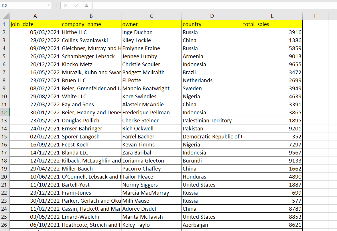
In the example below, we have a dataset of companies and their total sales in dollars for a particular day. Let’s say we want to aggregate the data by country of origin. For each country we should see the sum of all total sales as well as that amount after tax.
The Pivot Table below uses the Country field as a row label. In column C, we’ve added a calculated field that deducts a certain percentage from the sum of all sales in a particular country.
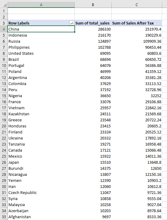
To get the values in Column C, we just need to use the following formula:
= total_sales - (total_sales * 12%)
You can make your own copy of the spreadsheet above using the link attached below.
If you want to try creating your calculated fields in Excel, simply follow our guide in the next section.
How to Add a Calculated Field to Pivot Table in Excel
This section will explain how you can start adding a calculated field to your Pivot Table. You’ll learn how to create a new Pivot Table from a dataset and define a new field.
Follow these steps to start adding calculated fields:
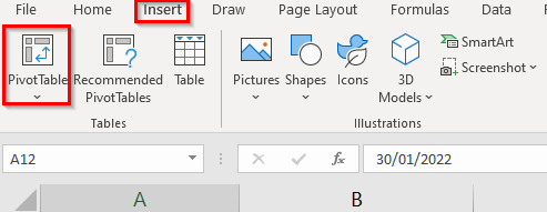
- In the Insert tab, click on the icon labeled ‘PivotTable’.
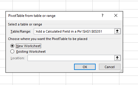
- In the new PivotTable dialog box, you can select a table or range to get data from. In this example, we’ll use the company sales data shown in the previous section. Click on the OK button.
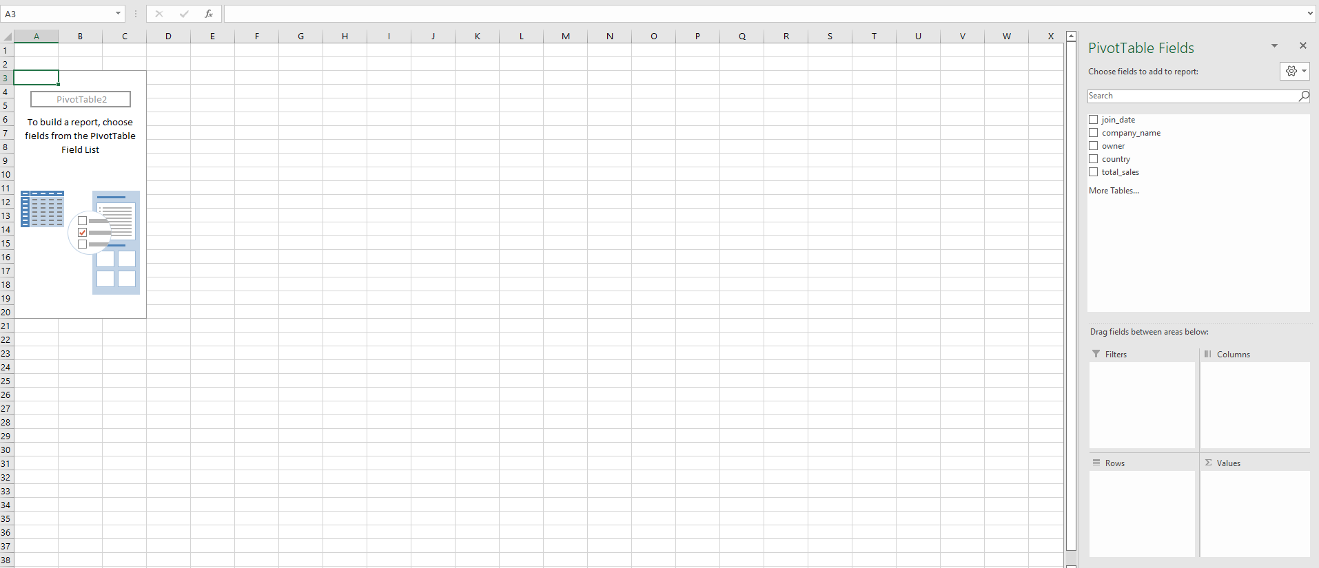
- Your spreadsheet should now have a Pivot Table and a Pivot Table Fields panel on the right-hand side of the screen. The panel should list down all available fields.
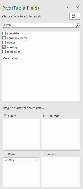
- For this example, we’ll first add the country field under the Rows area to group sales data later by region.
- Drag the total_sales field to the Values area. By default, the field should now be renamed Sum of total_sales. If this is not the case, users can manually change it by accessing the field’s settings.

- The Pivot Table should now have the sum of total sales per country.

- To add our new calculated field, go to the PivotTable Analyze tab and click on the Fields, Items, & Sets icon.

- From the dropdown menu, select Calculate Field.

- A new dialog box will appear. Users must name their new calculated field and define it with a formula that uses other fields. In the example below, we’ve created a new calculated field named Sales After Tax.

- Click on the Add button to add the calculated field to the Pivot Table. Once all necessary calculated fields have been added, click on OK.

- You can now add your new calculated field to your Pivot Table.
This step-by-step guide should be all you need to begin adding calculated fields to Pivot Tables in Excel. It should now be easy for you to start defining new fields using formulas through Excel’s Pivot Table Analyze tab.
Excel’s Pivot Table is just one example of a powerful tool you can use to explore your data. With so many other Excel functions available, you can surely find one that suits your use case.
Are you interested in learning more about what Excel can do? Subscribe to our newsletter to find out about the latest Excel guides and tutorials from us.