This guide will discuss how to group by month and year in a pivot table in Excel using two easy and simple methods.
The rules for using the YEAR function in Excel are the following:
- The
YEARfunction will return the year component of a selected date as a 4-digit number format. - The
YEARfunction only supports date values that are valid Excel dates. - When we input a text value, the function will return a #VALUE error.
Excel is an excellent tool for storing, organizing, and manipulating data. Since it has several built-in functions and tools, we can easily perform certain tasks to our data set, such as grouping data by month and year in a pivot table.
Luckily, we can easily group data by month and year since the pivot table has the features to group certain dates. In this case, we will utilize the group option of the pivot table to group data by month and year.
Additionally, we can create pivot table fields of months and years using the YEAR function, which we can simply display in the pivot table to group by month and year.
Let’s take a sample scenario wherein we have to group by month and year in a pivot table in Excel.
Suppose you are an employee of a company creating a sales report based on the last three years. And you want to be able to group the data by month and year in a pivot table to easily show and interpret certain data from a specific time period.
To do this, you used the group option of the pivot table to easily group the data by month and year.
Before we move on to a real example of grouping by month and year in pivot table in Excel, let’s first learn how to write the YEAR function in Excel.
The Anatomy of the YEAR Function
The syntax or the way we write the YEAR function is as follows:
=YEAR(serial_number)
Let’s take apart this formula and understand what each term means:
- = the equal sign is how we activate any function in Excel.
- YEAR() refers to our
YEARfunction. And this function is used to return the year of a selected date in the form of an integer in the range 1900 to 9999. - serial_number is the only required argument. So this is the number in the date-time code used by Excel.
Great! Now we can dive into a real example of grouping by month and year in a pivot table in Excel.
A Real Example of Grouping by Month and Year in Pivot Table in Excel
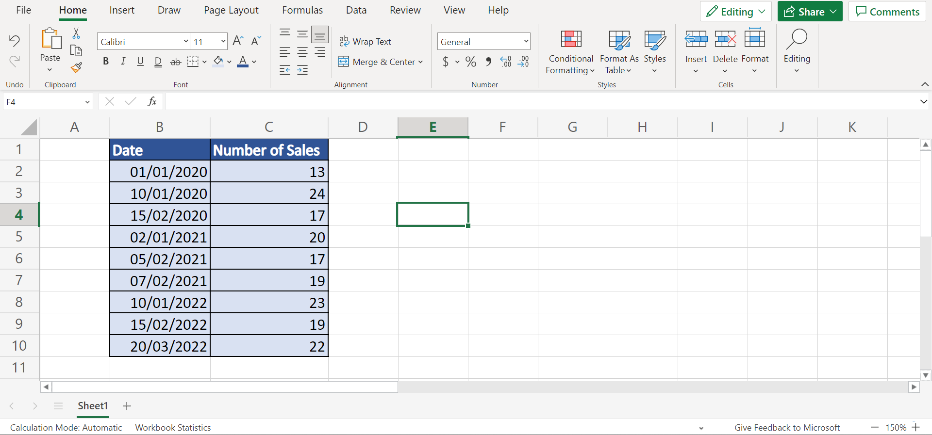
Let’s say we have a data set containing the dates of a sale from the last three years. And we want to group them by month and year in a pivot table. So our initial data set would look like this:
So we will utilize two easy and simple methods to do this task. Firstly, we can simply use the group option in the pivot table. However, we need to disable the automatic grouping option since the pivot table automatically groups data by dates in Excel.
After we disable this option, we can convert our data set to a pivot table. Then, we can add the necessary fields to display in our pivot table. Next, we can now use the group option to group the data by months and years. Additionally, there are several ways to do this grouping method. But, this is the easiest one.
Secondly, we can also create month and year columns for our data set. Then, we can use those columns as pivot table fields to display in our pivot table. And this will automatically group the date by month and year.
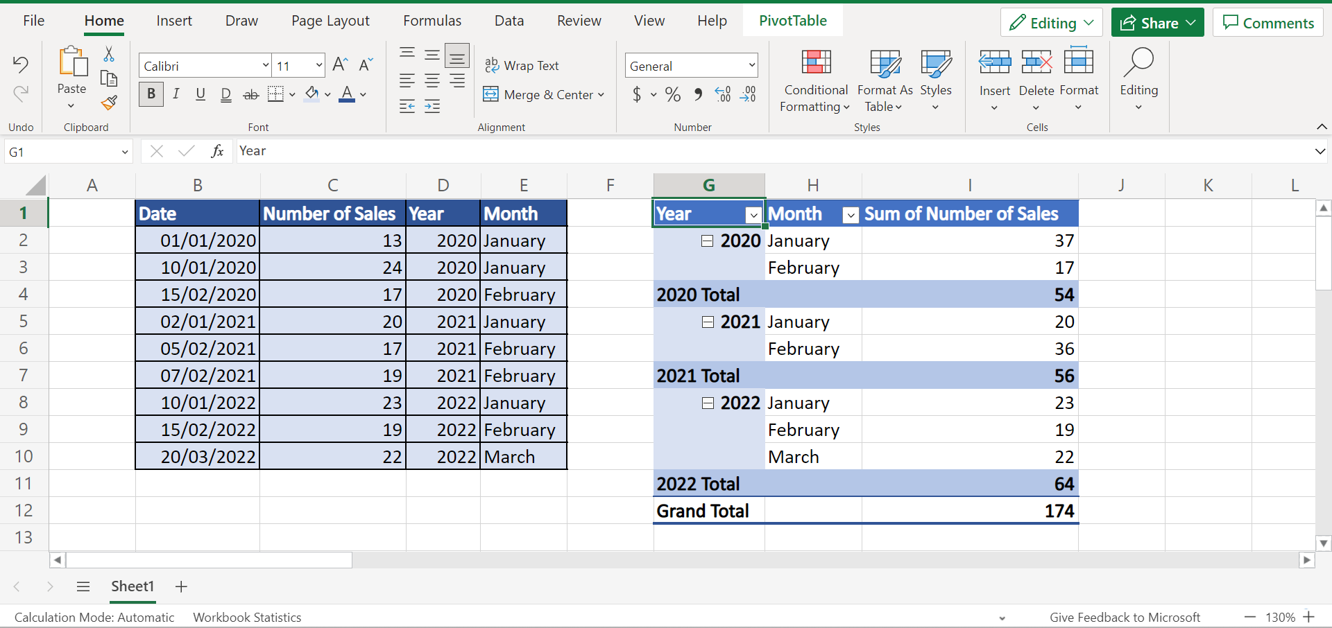
To do this, we will use the YEAR function to extract the year from each date. Then, the TEXT function will be used to extract the month from each date. When we convert our data set to a pivot table, we will have month and year pivot table fields to display.
So we only have to select the month and year fields. Then, the pivot table will automatically group the date by month and year. And our final data set would look like this:
You can make your own copy of the spreadsheet above using the link attached below.
Amazing! Now we can explain the process of how to group by month and year in a pivot table in Excel.
How to Group by Month and Year in Pivot Table in Excel
In this section, we will discuss the step-by-step process of how to group by month and year in a pivot table in Excel. Moreover, each step has detailed instructions and pictures to guide you.
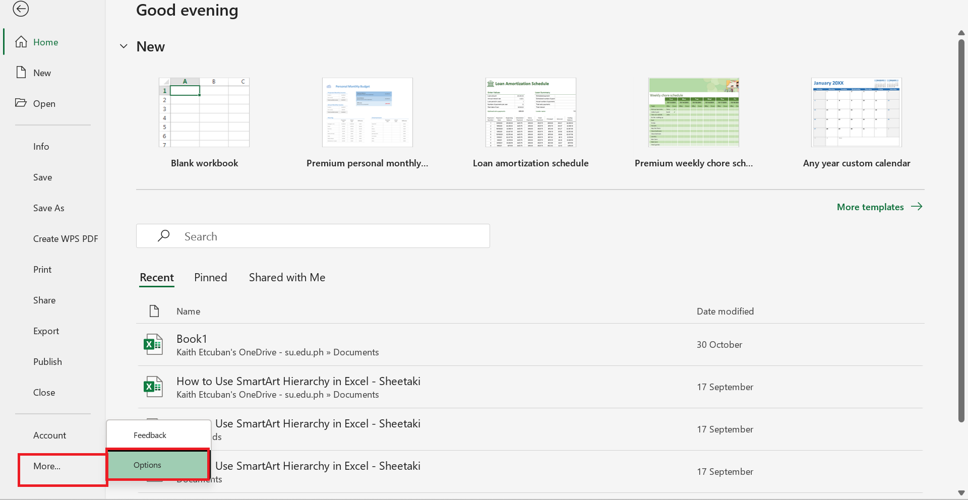
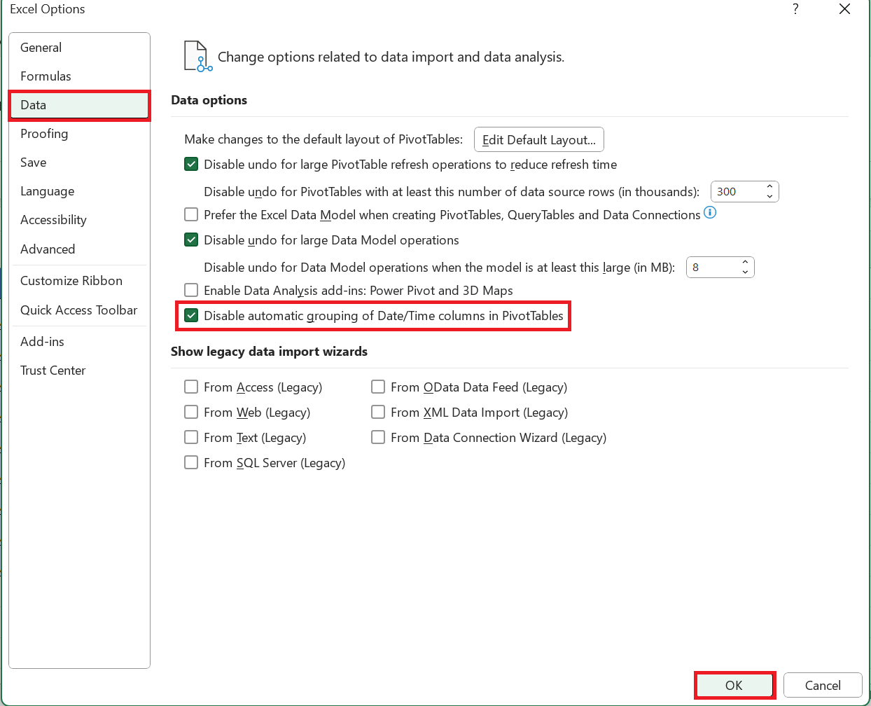
1. Firstly, we will use the group option. But, we first need to disable automatic grouping. So we will select File at the top left. Then, select More at the bottom of the page and click Options at the dropdown menu.
2. Next, we will go to the Data section and check the box Disable automatic grouping of Date/Time columns in PivotTable. Lastly, click OK to apply the changes.
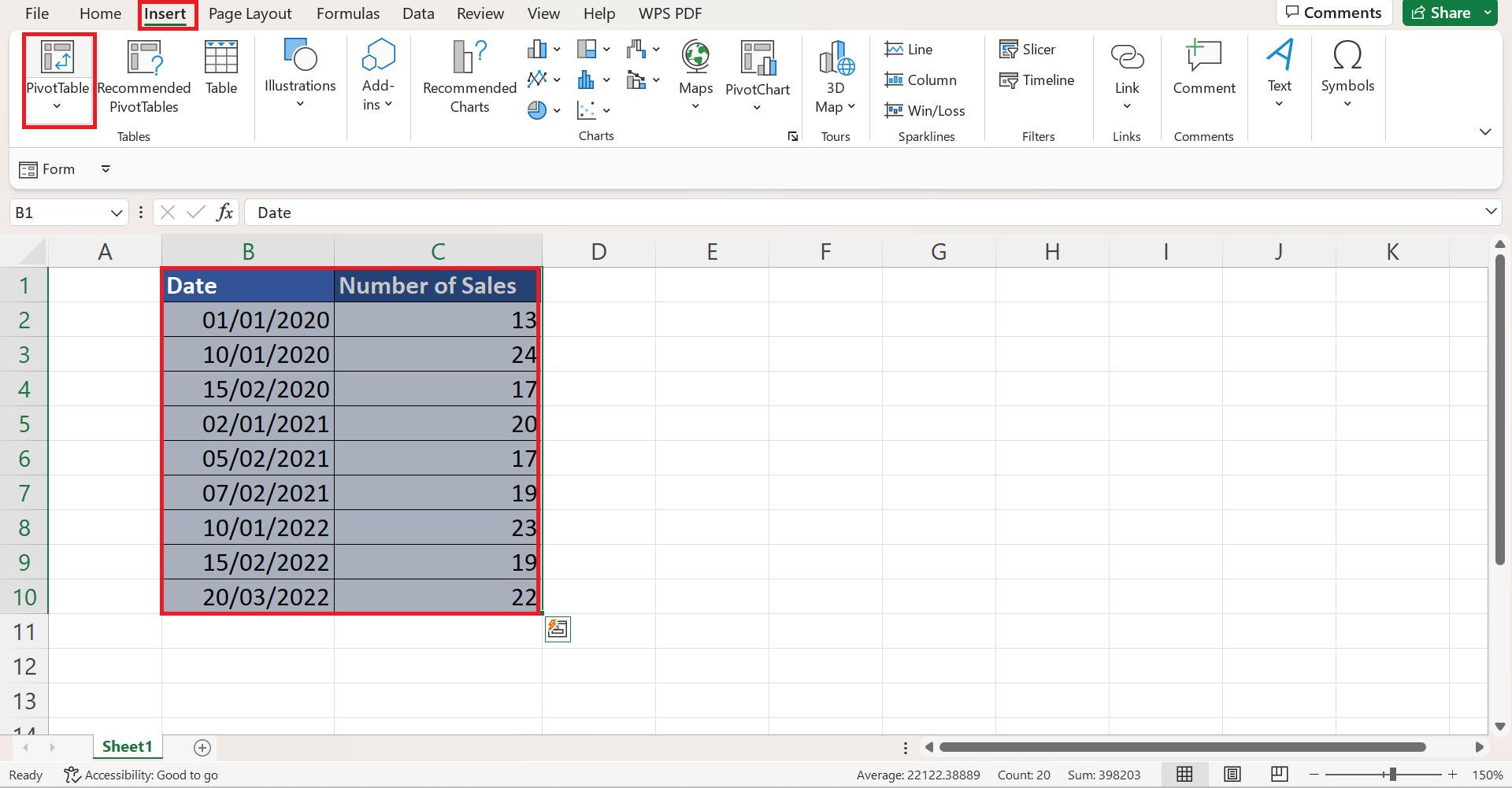
3. Now, we can convert our data set to a pivot table. To do this, we will select the entire data set and go to the Insert tab. Then, we will click PivotTable.
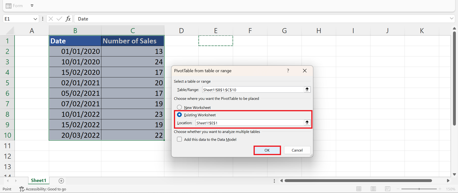
4. In the PivotTable from table or range window, we will select Existing Worksheet and input a cell location to display our pivot table. Finally, click OK.
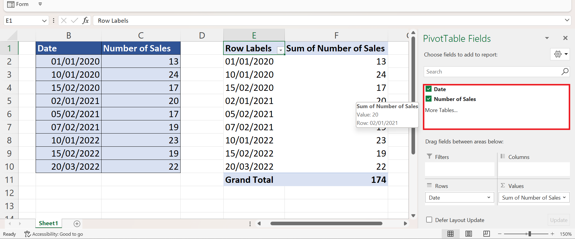
5. Then, we will select the Date and Sales to display or add them to our pivot table.
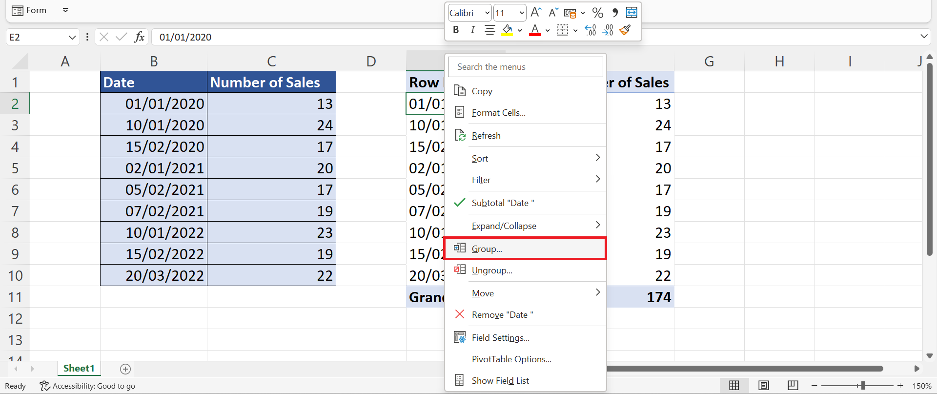
6. Afterward, we will select any cell in the pivot table and right-click. Next, we will click Group.
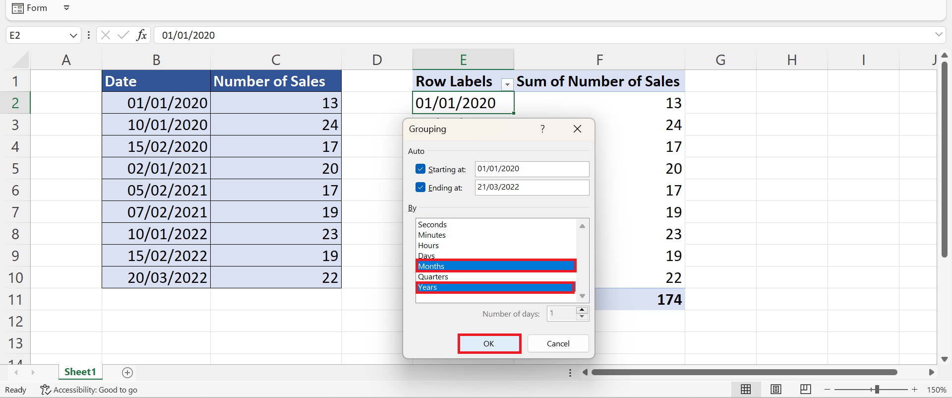
7. In the Grouping window, we will select Months and Years in the By section. Lastly, we will click OK to apply the changes.
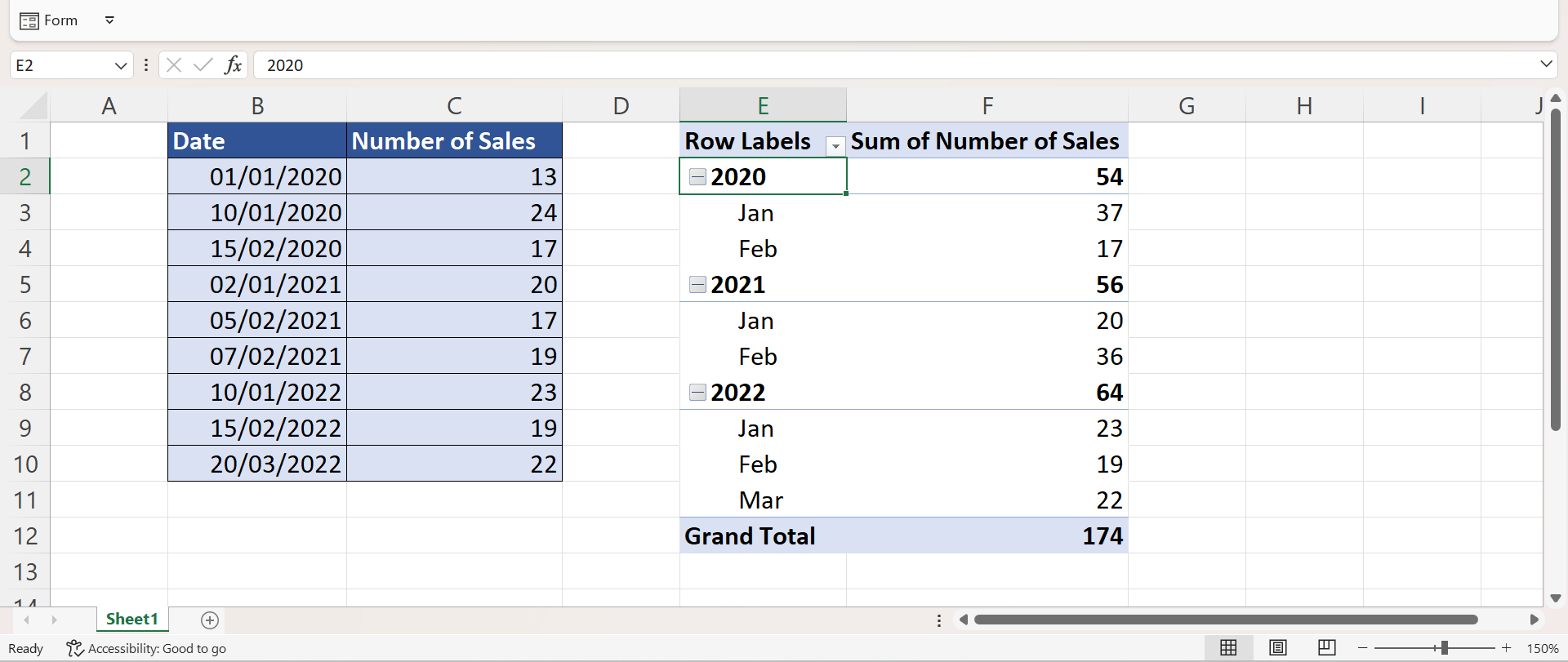
8. And tada! We have successfully grouped by month and year in a pivot table in Excel.
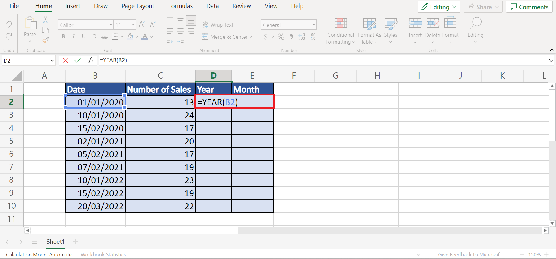
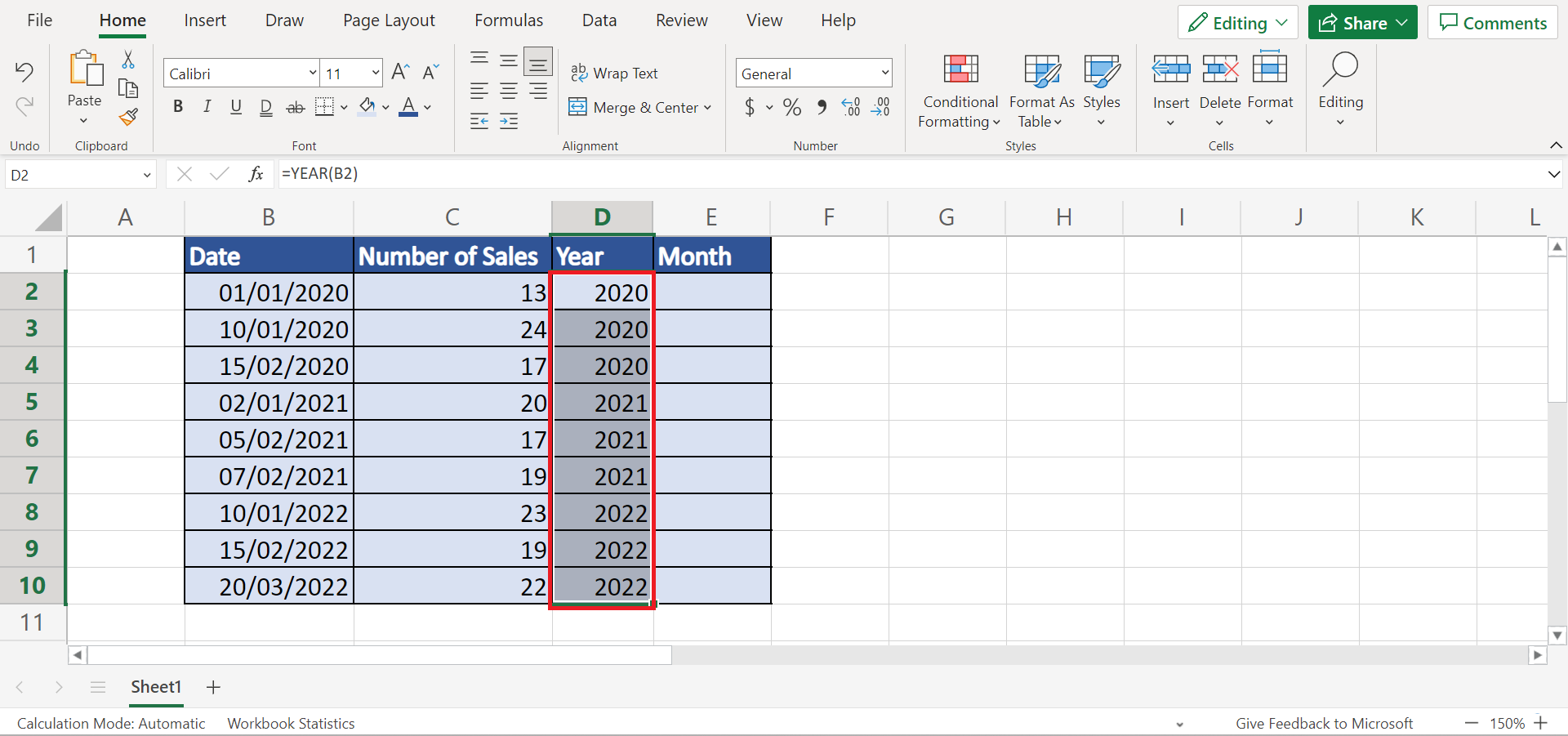
9. Secondly, let’s try another method to group by month and year in a pivot table. In this case, we will use some built-in functions to create new pivot table fields. So we will make two new columns for the year and month. Then, we will type in the formula “=YEAR(B2)” in the Year column.
Lastly, we will press the Enter key to return the result.
10. Then, we will drag down the Fill Handle tool to copy the formula to the rest of the column.
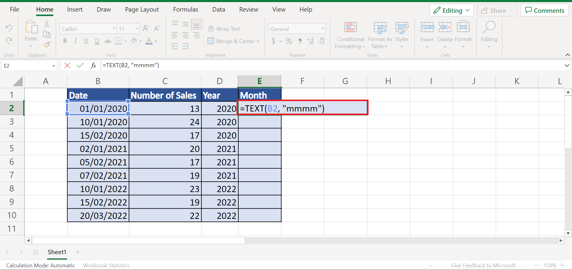
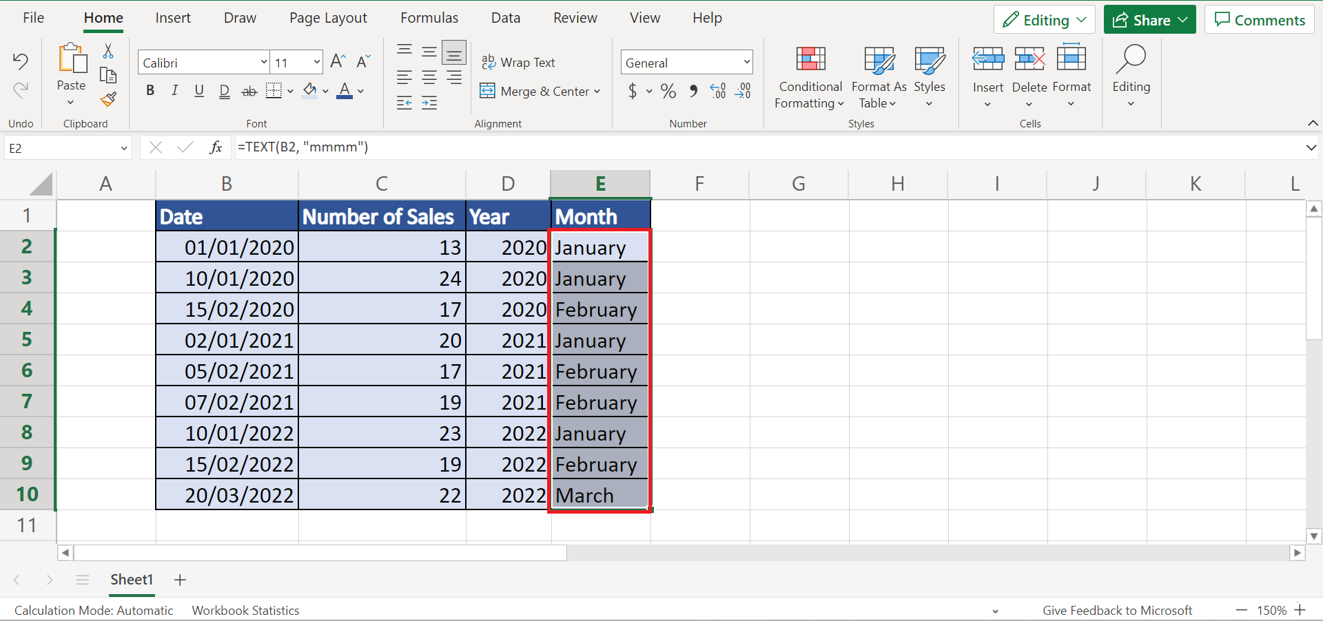
11. Next, we will use the TEXT function to extract the month from the dates. To do this, we will input the formula “=TEXT(B2, “mmmm”)” in the Month column. Lastly, we will press the Enter key to return the result.
12. Afterward, we will drag the Fill Handle tool down to copy and apply the formula.
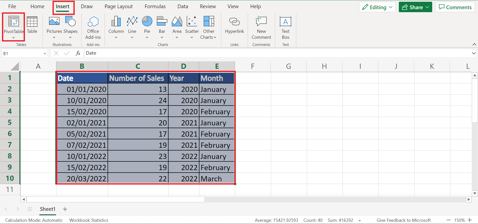
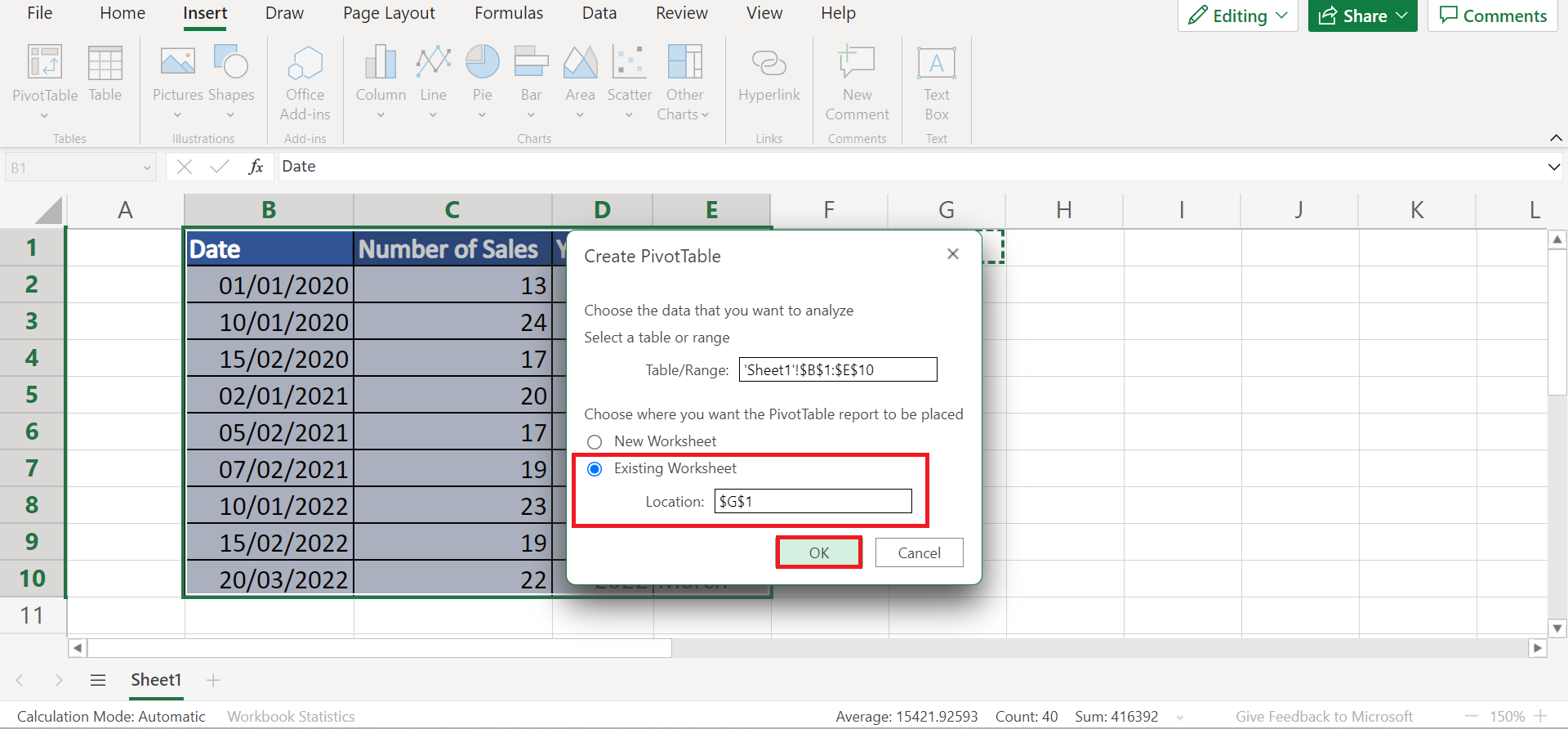
13. Then, we can now create a pivot table from the data set. So we will select the entire data set and go to the Insert tab. Next, we will click PivotTable.
14. In the Create PivotTable window, we will check Existing Worksheet and input a cell location.
15. After, we can simply check the fields to display them in the pivot table.
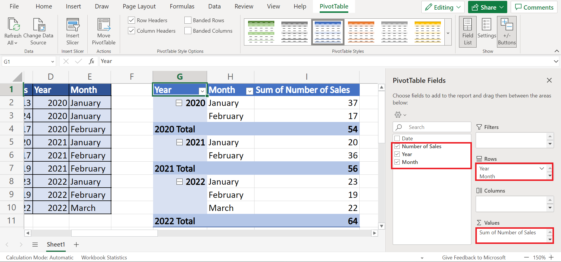
16. And tada! We have successfully grouped by month and year in a pivot table in Excel.
And that’s pretty much it! We have explained how to group by month and year in a pivot table in Excel using two easy and simple methods. Now you can choose any of the two methods and apply them to your work.
Are you interested in learning more about what Excel can do? You can now use the YEAR function and the various other Microsoft Excel formulas available to create great worksheets that work for you. Make sure to subscribe to our newsletter to be the first to know about the latest guides and tutorials from us.