How to Use MAXIFS Function in Google Sheets

The MAXIFS function in Google Sheets is useful to return the maximum value of a range based on one or more criteria.

The MAXIFS function does this by searching for the greatest number based on one or multiple conditions from the specified cells.

Let’s take an example.

Say we are creating a budget for our activities, and we want to find the most expensive things we purchased in each category. 💸

So how can we do that?

It’s easy. The MAXIFS function can return the greatest value from a data set filtered by multiple criteria.

The MAXIFS function does the exact opposite than the MINIFS function in Google Sheets that finds the minimum value in a range based on some criteria. Thus the way we use these two functions is very similar.

Now let’s dive into a few examples and get to know how the MAXIFS function in Google Sheets works.

The Anatomy of the MAXIFS Function

The syntax of a function specifies how we should use the function. The syntax of the MAXIFS function is almost the same as the MINIFS function.

The way we write the MAXIFS function looks like this:

=MAXIFS(range, criteria_range1, criterion1, [criteria_range2, criterion2, …])

Let’s break this syntax down and understand what these terms mean:

• = the equal sign is how we start each and every function in Google Sheets.
• MAXIFS is our function. We will have to add the corresponding variables into it for it to work.
• range is the range of cells from which we want to find the maximum value. It is a required field and should contain numeric values.
• criteria_range1 is the range of cells over which we want to evaluate a condition. It can be the same range as the original range or any other range of the same size.
• criterion1 is the condition we want to apply to the selected criteria_range1. The criterion will filter which cells should be considered to find the maximum.
• criteria_range2, criterion2 , ... are optional additional ranges and their associated criteria.

⚠️ A Few Notes to Make Your MAXIFS Function Work Perfectly

1. The shape and size of the range and all the criteria ranges must be equal. Otherwise, you will get an error value (#VALUE! error).
2. The MAXIFS function will return 0 if none of the criteria is satisfied.
3. While the range of the MAXIFS function must contain numeric values to get the maximum value, the criteria can be applied to dates, numbers, and text values as well.
4. It supports the use of logical operators (>,<,<>,=) and wildcards (*,?) in the criteria. The wildcards can be used to define partial matching.

Now let’s see some real-life examples where we can use our own MAXIFS function.

A Real Example of Using MAXIFS Function

Have a look at the picture below to see how the MAXIFS function in Google Sheets works.

MAXIFS Function with One Condition

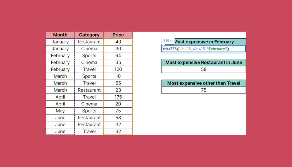
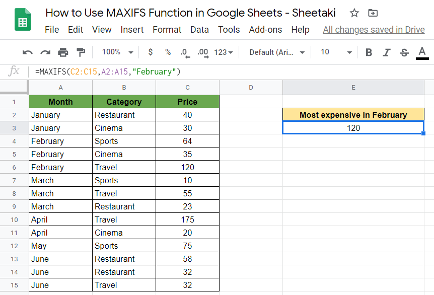
In the first example, we looked for the most expensive item of February.

The formula is as follows:

=MAXIFS(C2:C15,A2:A15,"February")

Here is what this example does:

• Firstly, we selected a cell where we wrote our MAXIFS formula. Here we selected the cell E3.
• We wrote a simple MAXIFS function with one condition. The first argument (C2:C15, in this example) is always the range in which we want to determine the maximum value.
• Then, we added the range/criteria pair of our MAXIFS function. The range of our criterion is the column of the months, so A2:A15.
• After that, we added the condition itself. We only looked within the rows that have “February” in this column, so this is our third argument in the function.
• As a result, we got 120, which is the price of our most expensive item in February indeed.

Simple, isn’t it?

You can make a copy of the spreadsheet using the link attached below and have a try:

MAXIFS Function with Multiple Conditions

We can add more conditions to our MAXIFS function in a simpler and straightforward way.

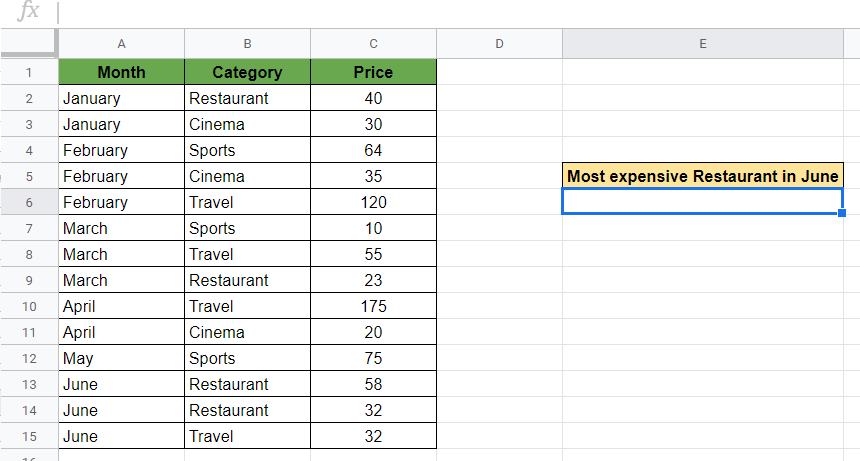
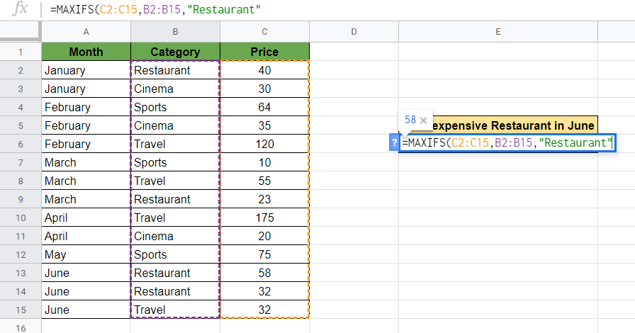
The picture below shows how we found the most expensive item of “June” that is in the “Restaurant” category.

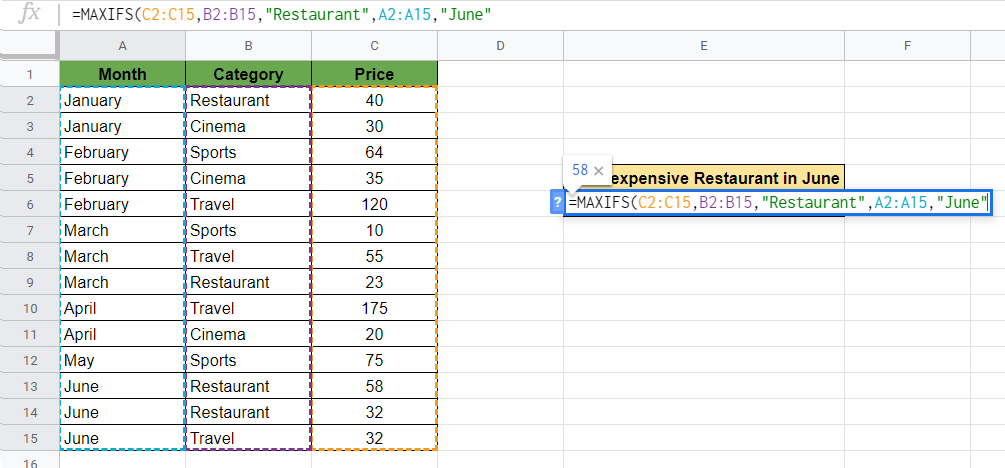
The function now has one more range/criteria pair, and it’s written as follows:

=MAXIFS(C2:C15,B2:B15,"Restaurant",A2:A15,"June")

Here’s what this example does:

• The range is the same as before (C2:C15), which is the area of prices.
• We added our first criteria_range1, which is the ‘Category’ column (B2:B15).
• Then, we added the criterion to this range, which is “Restaurant”. We only wanted to consider the items that are in this category.
• After that, we added a second criteria_range2. Now we wanted to search for the months, so it’s the range A2:A15.
• We added the criterion2 that we wanted to apply to this criteria range. We filtered the expenses of June, so our criterion2 is “June”, always written in double-quotes.
• As a result, we got 58. This is the price of the most expensive restaurant visit we had in June.

Following the way we showed here, we can even more conditions to our function and filter our results by many criteria. The order of the conditions doesn’t matter, because they will all be evaluated.

MAXIFS Function with Operators

When writing the criteria of our MAXIFS function, we can set more complicated conditions than just simple equality checks.

In the next example below, you can see how to write a condition with an operator.

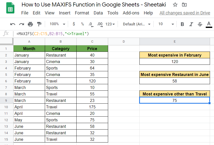
Here we retrieved the highest price from all the expenses that are not in the “Travel” category.

The function is as follows:

=MAXIFS(C2:C15,B2:B15,"<>Travel")

By now, you have already seen how to select the range (Prices, C2:C15) and the criteria_range1 arguments (Category, B2:B15).

The interesting new part is the third argument:

"<>Travel"

We used the ‘<>’ comparison operator that is the Not equal operator. We can use it when we want to have the value in a cell not to be equal to the term we write next to it.

So in this example, we ruled out all the rows that are in the Travel category and only considered the remaining rows. Out of these rows, 75 is the greatest number indeed that the function outputs as a result.

Similarly, you can use any other operators in your functions, for example:

• ‘<’ less than,
• ‘>’ greater than,
• ‘<=’ less than or equal,
• ‘>=’ greater than or equal,
• ‘=’ is equal to.

Now let’s begin writing your own MAXIFS function in Google Sheets step-by-step.

How to Use MAXIFS Function in Google Sheets

1. To begin, select a cell where you want to output the result. For this guide, we will be writing our MAXIFS function in cell E6.

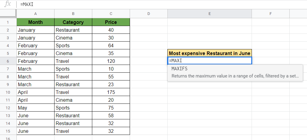
2. Start typing an equal sign ‘=’ and the name of the function which is MAXIFS. Select the right function from the auto-suggest box that will open your opening bracket ‘(‘ automatically.

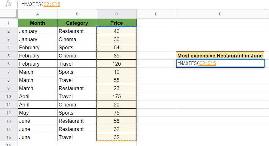
3. Then, you have to add the first argument. The range is the column with numeric values from which you want to retrieve a maximum value. In our example, we will be selecting the range of C2:C15, where we have the prices.

4. After that, add a comma, and then the first range/criteria pair you want to define. Select the criteria_range1 first that must be of the same shape and size as your range. We will be selecting the range of ‘Category’, which is the range B2:B15.

5. Now, add the condition to this range as the criterion1 variable. We will be adding the condition “Restaurant” because we want to look for the maximum value in this category. Make sure to write the condition exactly as it is in the sheet because the function only checks for 100% equality.

6. Then, you may add more conditions to the function. For our example, we will be adding a second range and condition to filter the expenses from June. So, the criteria_range2 argument will be the column of ‘Month’, which is the range of A2:A15.

7. Next, add the condition that you want to filter by in this second range. We will be writing ”June” within double-quotes to set the criterion2.

8. You may add a third condition and even more if you would like to filter your results even more.

9. Finally, after you have added all the conditions you wanted to, close the brackets ‘)‘ and hit the Enter key. As a result, you should see the maximum value based on all the conditions you set.

That’s it, well done! You can now use the MAXIFS function together with the various other Google Sheets formulas to create even more useful formulas. 🙂

Get emails from us about Google Sheets.

Our goal this year is to create lots of rich, bite-sized tutorials for Google Sheets users like you. If you liked this one, you'll love what we are working on! Readers receive ✨ early access ✨ to new content.

Subscribe