How to Use SEQUENCE Function in Google Sheets

The SEQUENCE function in Google Sheets is useful to return an array of sequential numbers vertically or horizontally. You can create single or multiple columns sequences as well as define a step value.

The SEQUENCE function does this simply by taking the number of rows, column, starting number, and step value and create an arithmetic sequence.

Arithmetic sequence means that the difference between one term and the next is a constant. In other words, we just add the same value each time. For example, 1, 3, 5, 7, and so on.

So how do we do that?

The SEQUENCE function only needs the starting criteria of the sequence, and it fills the whole list (or a multiple columns table) of numbers automatically. In conclusion, you only need to write the function in one cell, and it will provide the whole sequence.

Let’s dive right into real examples to see how to use SEQUENCE function in Google Sheets.

The Anatomy of the SEQUENCE Function

So the syntax (the way we write) the SEQUENCE function is as follows:

=SEQUENCE (rows, columns, start, step)

Let’s dissect this and understand what each of these terms means:

• = the equal sign is just how we start any function in Google Sheets.
• SEQUENCE is our function. We will have to add the
• rows variable(s) into it for it to work.
• rows is the required field that represents the number of rows to return.
• columns is an optional field that represents the number of columns to return. If you omit using it, the returned array will have 1 column.
• start is an optional field that represents the number to start the sequence at. If you omit using it, the sequence will start at 1.
• step is an optional field that represents the amount to increase (or decrease) each number in the sequence. By default, it will increase the sequence by 1.

You can create sequences with different structures with the SEQUENCE function. Above all, it depends on how you use the variables (the required and optional fields of the function).

• If you only give the number of
• rows in your function and omit using the rest of the variables, you get a single vertical list of numbers starting from 1. The formula below creates a sequence of one column with three rows.

=SEQUENCE(3)

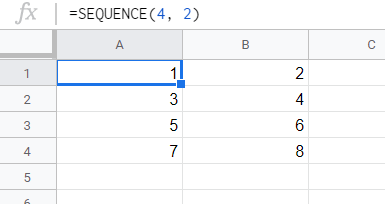
• Now let’s see how to create sequences with multiple columns. The first two variables mean that you define the number of
• rows and columns. This solution creates a table with four rows and two columns.

=SEQUENCE(4, 2)

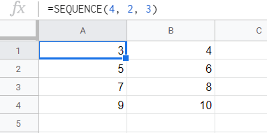
• You can give a third variable start to define which number to start the sequence with. This way, it doesn’t start with the default 1, but with 3.

=SEQUENCE(4, 2, 3)

• The last variable is the step value. Instead of increasing the numbers by 1 in the sequence, you can set any other number to increase (or decrease) it. With the formula below, the sequence has a difference of 2 between each number.

=SEQUENCE(4, 2, 3, 2)

There are a lot of ways to create sequences with this function. Additionally, there are some special use cases of it, which you can see under the notes below.

⚠️ A Few Notes to Use SEQUENCE Function Even Better

1. step value can be negative, and you can create sequences with decreasing order.
2. You can create single row horizontal sequences when setting the number of rows to 1.
3. You can easily create a single column list of numbers without the use of SEQUENCE function. This can be done by entering at least two values next to each other, highlighting them, and then dragging the blue highlighting box down or across. However, there is a difference when you want to insert or delete a row from the sequences. The SEQUENCE function always results in a continuous list, meanwhile, the drag-down solution can be interrupted.
4. There is an identical solution to the SEQUENCE function with the combination of ROW and ARRAYFORMULA. The formula =SEQUENCE(5) gives the same result as =ARRAYFORMULA(ROW(A1:A5)
5. Dates and times are considered numbers in the background. This means that it’s possible to create sequences of dates and times with the SEQUENCE function. You can give a date as the start variable with a simple DATE function.

=SEQUENCE(4, 2, DATE(2020, 4, 1), 1)

You just need to format the result from numbers to dates. Select the whole area with the sequence and click on Format > Number > Date.

A Real Example of Using SEQUENCE Function

Take a look at the example below to see how SEQUENCE functions are used in Google Sheets.

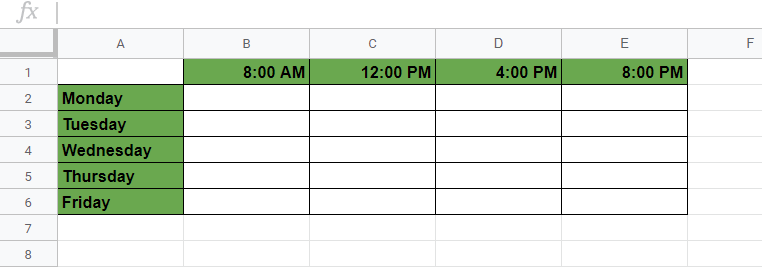
Say we are creating a sheet to count how many products are created in a shoe factory in one week. 👟

The working hours are from 8 AM to 8 PM from Monday to Friday. One thousand pairs of shoes are produced every 4 hours.

We want to see how many pairs of shoes should be in the inventory at 8 AM, 12 PM, 4 PM, and 8 PM each day. Thus we want to create a sequence that calculates the exact number of shoes at these moments.

We fill the SEQUENCE function with the right variables:

• The table goes from Monday to Friday, so the number of rows is 5.
• Then, there are 4 columns with the indicated times in the top row.
• The next variable is the start, which is 0 because there are no shoes produced at the beginning of the first day.
• Finally, we need to define the velocity of the production. In other words, how many pairs of shoes are produced every 4 hours? The step is 1000 in this example.

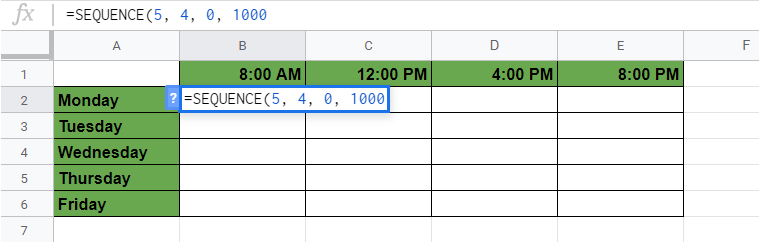
To put this all together, the SEQUENCE function we write in cell B2 is this one:

=SEQUENCE(5, 4, 0, 1000)

After hitting the Enter key, we can see the number of shoes in the inventory throughout the week:

Super easy, right?

You can change the variables in the first cell of the sequence, and it will change the whole sequence. For example, you can change the velocity of production (the step variable) from 1000 to 1500, and the entire table is recalculated accordingly.

Try it out by yourself. You may make a copy of the spreadsheet using the link I have attached below and try it for yourself:

How to Use SEQUENCE Function in Google Sheets

Let’s see how to use SEQUENCE function in Google Sheets step-by-step.

1. To start, simply click on any cell to make it the active cell. For this guide, I will be selecting B2, where I want to show my result.

2. Next, type the equal sign ‘=’ to begin the function and then followed by the name of the function which is ‘sequence (or ‘SEQUENCE‘, whichever works).

3. Great! Now you should find that the auto-suggest box will pop-up with the name of the function SEQUENCE.

4. After the opening bracket ‘(‘, you have to add the variables. Remember that you can add up to 4 variables, but only the first one (rows) is required, the rest are optional. In this example, we have five rows (from Monday to Friday) and four columns with the times. Therefore, we create a sequence of 5 rows and 4 columns. So the first two variables are 5 and 4.

5. After that, we need to define the start of our sequence, which is 0. This is the next variable in the function.

6. Finally, we have to add the step value. We want to increase the numbers by 1000 each cell, so we write 1000 as the last variable.

7. Hit the Enter key, and you can see the whole table with the sequential numbers!

That’s it, good job! You can now use the SEQUENCE function together with the other numerous Google Sheets formulas to create even more powerful formulas that can make your life much easier. 🙂

Get emails from us about Google Sheets.

Our goal this year is to create lots of rich, bite-sized tutorials for Google Sheets users like you. If you liked this one, you'll love what we are working on! Readers receive ✨ early access ✨ to new content.

Subscribe