How to Use QUERY Function in Google Sheets

The QUERY function in Google Sheets is one of the most powerful functions as it is useful for all your needs – logical, lookup, summation, and counting. You could even use it when you are averaging, filtering, and sorting.

The QUERY function does this simply by adding the criteria. The function automatically outputs the data you want to see based on the criteria.

Let’s take an example to understand the concept better.

Say we need to sort the students for us to determine who among them will go to the Best Class. For a student to be in the best class, his/her grade should be above 89.

So how do we do that?

Simple. Let’s determine the given. The students’ record is our data, and ‘above 89‘ is our criteria. We will then supply our QUERY function with the needed attributes.

Ultimately, our QUERY function will output the name of the student. If you want our function to output an ID number or the age, maybe, these are all possible. You just have to tweak the syntax a bit to make it work smoothly.

See how easy that is?

Indeed, you can do a lot of things with this QUERY function as it is one of the most powerful functions in Google Sheets, and of course, one of the coolest tools to have in your Sheetaki arsenal to solve a lot of your business data entry problems.

Let’s dive right into real-business examples where we will deal with actual values and textual strings and how we can write our own QUERY function in Google Sheets to compute those data.

The Anatomy of the QUERY Function

So the syntax (or the way we write) the QUERY function is as follows:

=QUERY(data, query, [headers])

Let’s break this down into pieces to understand better what each terminology means:

• = the equal sign is just how we usually start any function in Google Sheets.
• QUERY() is our function. We still need to add the data and query attributes for it to work.
• data is the range of cells where you want to query upon. This serves as the syntax’ reference.
• query is the reference to a cell where the query is placed. When writing your query, it should be enclosed in a quote-unquote symbol as it is a text string. We can also consider this as our criteria.
• [headers] is optional. This tells the number of header rows at the top of the data.

⚠️ Now a few notes before writing your own QUERY function.

1. You must enclose your query attribute in a quote-unquote symbol, (” “).
2. You can use comparison operators in your query attribute. Comparison operators are the following:
   • greater than, >
   • less than, <
   • equal to, =
   • not equal to, <>
   • greater than or equal to, >=
   • less than or equal to, <=

3. Depending on how large your data is, you might need more space just below the cell where you’ve written your QUERY formula.

A Real Example of Using QUERY Function

Take a look at the example below to see how QUERY function is used in Google Sheets.

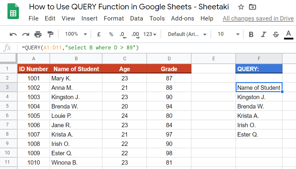
As you can see in the data above, the QUERY function is used to determine who among the students are qualified to be in the Best Class. The function outputs the names of qualified students. The function is as follows:

=QUERY(A1:D11,"select B where D > 89")

Here’s what this example does:

• We have actively selected the cell where we want to write our formula, and we want to use the QUERY function to determine who among the students are qualified.
• We select the data A1:D11, and this serves as our reference.
• Then, we added our query. Remember that we only want to have the names of the students whose grade is above 89. The names of the students are in column B. While the grades are in column D.
• Notice that in our query attribute, we used greater than (>) as our comparison operator. This is so because we wanted to get those with grades above 89, or greater than 89. That is also the same as saying, 90 and above.

Easy, right?

Try it out by yourself. You may make a copy of the spreadsheet using the link I have attached below:

Let’s begin writing our own QUERY function in Google Sheets.

How to Use QUERY Function in Google Sheets

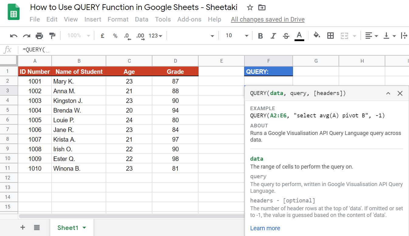
1. Simply click on any cell to make it active. This is where we want to write our formula. For this guide, I have selected cell F3.

2. Next, type in the equal sign “=” to start the function and then followed by our function, which is QUERY.

3. Wait for the auto pop-up message. This will serve as your extra guide in writing the formula.

4. Then, we select our data range. For this guide, I have selected A1:D11.

5. Great! The next step is to write the query. Begin this part by writing a quote-unquote symbol, (” “).

6. Inside the symbol, write select, followed by the column where your needed information is. For this guide, I want to output the name of the students. Therefore, I have written column B.

7. Still under the query attribute, right after adding column B, we need to add our ‘criteria‘, where D > 89. This would simply mean that our QUERY function will have to check those grades that are greater than 89. The grades can be found in column D.

8. Lastly, close your formula with a close parenthesis “)“, then hit on the ‘Enter’ key.

Bonus

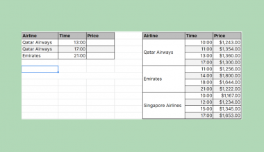
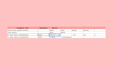
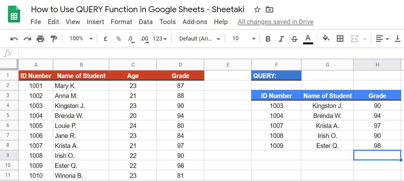
There might be a time when you want to output more than one information. Say, the ID number, and the Name of Student. If you want to output more than one information, simply add the column right after ‘select‘ in the query attribute part of the formula. The working formula would have to be:

Get emails from us about Google Sheets.

Our goal this year is to create lots of rich, bite-sized tutorials for Google Sheets users like you. If you liked this one, you'll love what we are working on! Readers receive ✨ early access ✨ to new content.

Subscribe