How to VLOOKUP Multiple Columns in Google Sheets

The VLOOKUP multiple columns in Google Sheets is useful if you want to pull out data from a complex database or tables.

The VLOOKUP does this in 3 different ways:

1. Combining search criteria
2. Creating a helper column
3. Using the ARRAYFORMULA function

The downside of the VLOOKUP function is, it can only have a single match. Meaning, if we want to check multiple columns, we have to combine the required data or pair the VLOOKUP function with other functions.

Let’s take an example.

Say we run a lending company. As of the moment, we have 100 borrowers, and we want to check how much each borrower owes.

So how do we do that? Easy. Using the various methods below, we can figure out how to check how much each borrower owes using the VLOOKUP function. We will show you how to implement each of the methods in the section “How to VLOOKUP Multiple Columns in Google Sheets” down below in this post.

---

Method # 1: Combining Search Criteria

If in case the database is presented in a manner that the first name and last name are combined in one cell, we need to sort and separate them. One column for the first name, and another for the last name. After sorting it out, we will now perform the VLOOKUP function. We supply the attributes needed for our function to work seamlessly.

---

Method # 2: Creating a Helper Column

If the database is presented in a way that the first name and last name are already separated, then this method is a more appropriate approach. This method requires you to create a helper column. All you need to do is combine the necessary columns in a new search column, that we now call the helper column. In this case, our helper column would be a combination of the first and last name. Basically, this method is the opposite of the previous one.

After creating a helper column, we’re now ready to perform the VLOOKUP function. We supply the required attributes, and it does its magic perfectly!

---

Method # 3: Using the ARRAYFORMULA Function

This method is in contrast with Method 2 above. Instead of creating a helper column, you can make use of the ARRAYFORMULA function. There are three main steps to do if you opt to go for this method. The steps are the following:

• Create an array of criteria columns. We need to generate an array of full names, which is first name + last name.
• After this, we add the remaining columns from the original database.
• We’re now ready to perform the VLOOKUP function.

In all the steps mentioned above, we will make use of the ARRAYFORMULA function.

Again, this was just a brief overlook of the various ways we can solve our problem. It may seem confusing at this point, but rest assured that we will go through each method step-by-step to learn precisely how to VLOOKUP multiple columns in Google Sheets.

Let’s dive into real-business examples to show you how we can write our own VLOOKUP function in Google Sheets to compute those data.

 

 

The Anatomy of the VLOOKUP Function

So the syntax (the way we write) the VLOOKUP function is as follows:

=VLOOKUP(search_key, range, index, [is_sorted])

Let’s break this down into pieces so we’d better understand what each terminology means:

• = the equal sign denotes the start of the function, just like any function in Google Sheets.
• VLOOKUP is our function. For the VLOOKUP() we will need to provide the attributes search_key, range and index to make it work.
• search_key is the value we are searching for.
• range is the array that we consider for the search
• index is the column of the value to be returned
• [is sorted]is optional. This indicates whether the column to be searched is sorted.

 

 

A Real Example of Using VLOOKUP Function

Take a look at the example below to see how VLOOKUP function is used in Google Sheets.

 

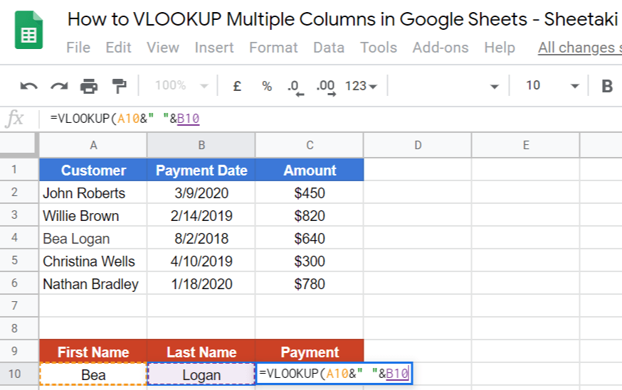
The above image shows how to VLOOKUP multiple columns in Google Sheets using the first method, which we had discussed in the beginning part of this post. The function is as follows:

=VLOOKUP(A10&" "&B10,A1:C6,3,false)

Here’s what this example does:

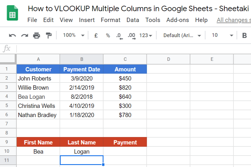
• As you can observe in our database, the first and last names were combined in one cell. So, we have separated them. We have column A for the first name, column B for the last name, and column C for the payment.
• Next, we actively selected an empty cell because this is where we will write our formula. For this guide, we picked cell C10.
• Then, we used our VLOOKUP formula to check Bea Logan’s payment.
• We supplied our formula with the necessary attributes, such as the first name (A10), the last name (B10), the database range, the index, and if the column to be searched is sorted or not (In this case, it’s not. Therefore, it’s False.)
• After we hit on the Enter key, it gave us an answer of $640, the same amount as what we had in our original database.

Easy, right?

Try it out by yourself. You may make a copy of the spreadsheet using the link I have attached below:

 

 

How to VLOOKUP Multiple Columns in Google Sheets

As promised, in this section, we will show you a step-by-step process on how to VLOOKUP multiple columns in Google Sheets, which will comprise of all the three methods that were discussed earlier. We will be using the same information as above: “We want to check how much did Bea Logan paid.”

Method # 1:

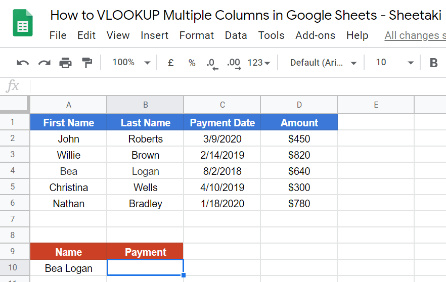
1. First, we need to separate the first name and the last name. For this guide, we have placed it just below the original database.

 

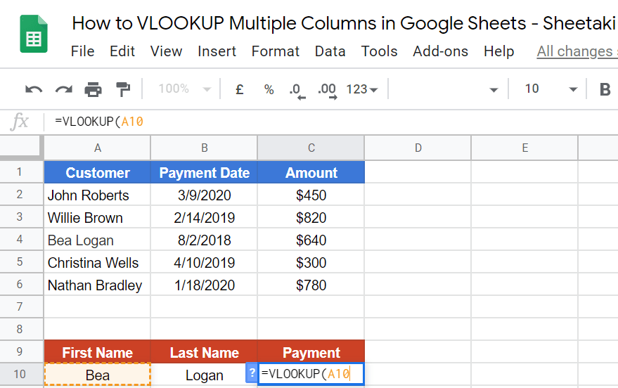
2. Next, we clicked on an empty cell to activate it. This is where we will write our formula. For this guide, we selected cell C10. We then started our formula by writing our function, which is VLOOKUP, followed by an open parenthesis ‘(‘.

 

3. Wait for a pop-up message, as this will give us an extra guide in writing our formula.

 

4. We selected cell A10 (first name).

 

5. After this, we added concatenated values &” “& to work as our first argument.

 

6. Then, we selected cell B10 (last name).

 

7. Next, we added the database range, which is A1:C6.

 

8. We followed it up with an index, 3. This is where our VLOOKUP function should get our desired answer. Then, we added ‘false‘. False signifies that our database isn’t sorted.

 

9. Lastly, hit on the Enter key, and you should find that the value $640 will be populated.

 

---

Method # 2:

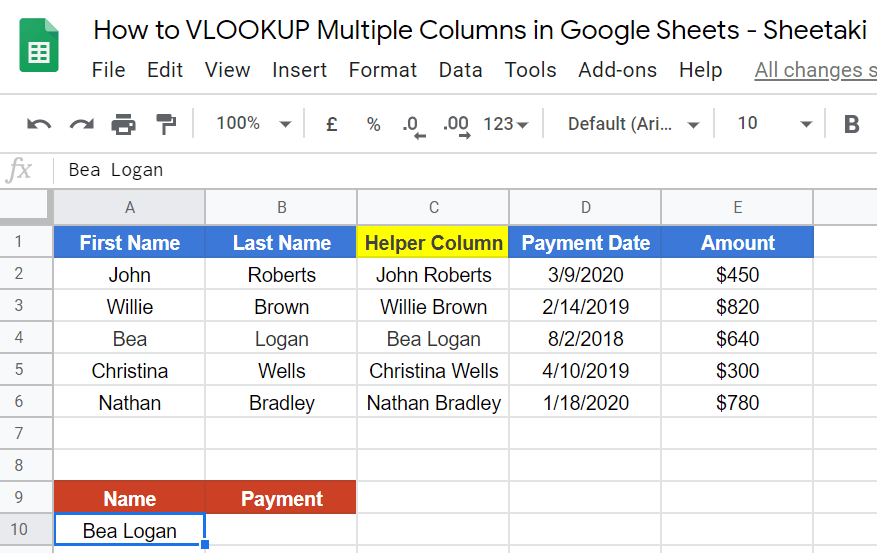
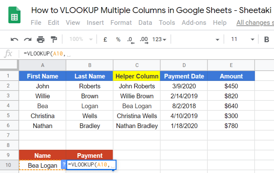
1. First and foremost, you will want to create a helper column. In our helper column, we just need to combine the first and the last name in one cell.

 

1. Since we want to check Bea Logan’s payment, we need to put her name in the cell A10, just below the ‘Name‘.

 

2. Next, we now activate an empty cell. This is where we will write our formula. For this guide, I’ve selected cell A10. Then moved forward to write our function, which is the VLOOKUP, followed by an open parenthesis “(“. Wait for an auto pop-up message that will serve as our guide in writing our VLOOKUP function.

 

3. Then, we will select cell A10 under the Name column.

 

4. Now, we select our database range. Since we’ve already created a helper column found in column C, we can already disregard columns A and B. So, we will only select the range C1:E6.

 

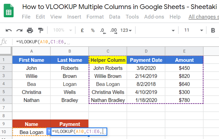
5. After that, write 3 because column 3 will serve as our index. Next, we follow by adding the word ‘false‘, because our database isn’t sorted out.

 

6. Hit on the Enter key, and you will get $640.

 

---

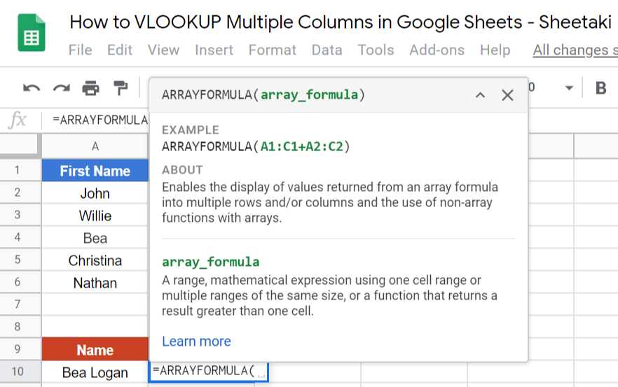
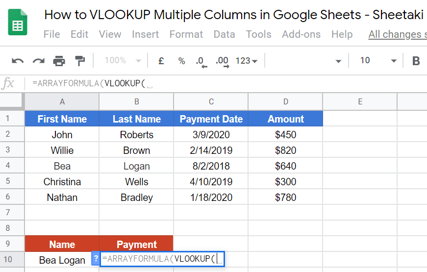
Method # 3:

1. Simply click on an empty cell to make it active. For this guide, I’ve selected cell B10.

 

2. Next, we will start our formula with the ARRAYFORMULA function.

 

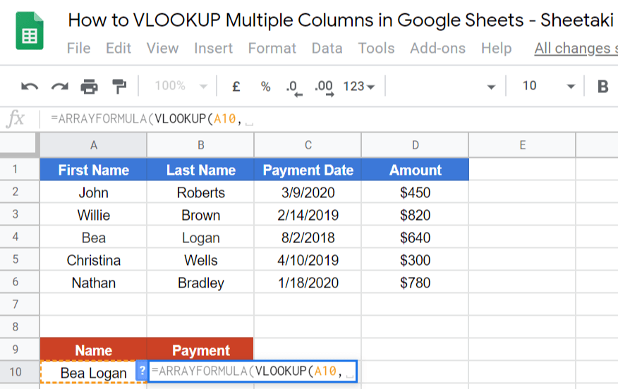
3. We follow it up with our VLOOKUP function.

 

4. Then, we carefully select the name. In our case, we choose A10.

 

5. After that, we need to add an open brace “{“, followed by the array in column A, and concatenated values &” “&.

 

6. We will then select the array in column B.

 

7. Next, we have to select the range C2:D6. Remember to NOT include the labels.

 

8. Close the brace “}“, then, we’ll finalize our formula by adding the index, which is 3, and the word ‘false‘ which signifies that our database isn’t sorted. Close the formula with two closing parentheses “))“.

 

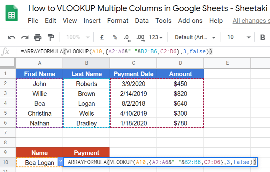
9. Hit on the Enter key. Voila! You should get $640.

 

That’s pretty much it. You can now use the VLOOKUP function together with the other numerous Google Sheets formulas to create even more powerful formulas that can make your life much easier. 🙂