The DSUM function in the Google Sheets formula is very similar to the SUM function, but with one exception. It gives us the sum of values in any numeric field in a database, based on the given condition(s). This is analogous to a SQL database sum query. The ‘D’ in the DSUM stands for ‘Database’. Therefore, we can call this a Database SUM formula.
DSUM is similar to another Google Sheets function called SUMIF/SUMIFS. Both of these can give you similar results depending on how you use them. For a more comprehensive guide on how to use the SUMIF/SUMIFS functions in Google Sheets, refer to our article on the same.
There is one difference, though. While the former is a database function that would return the sum of values selected from a database table similar array/range using an SQL like query, the latter is of a more logical type.
Let’s take an example.
While tracking my monthly expenses for June, I realized that the net spending was more than what I had expected. The particulars have been tagged under different categories, but I want to identify the net spending split into different categories, such as groceries, medicine, fuel, maintenance etc. Since the number of transactions is so large, it is cumbersome to individually add up each amount for every category.
This is where DSUM comes to my rescue. Because I already know the name of the category, I can simply refer to it and add all of the numerical values together in the same data structure.
That’s just one example. There are plenty of other use-cases for this function in real life. Great! Let’s dive right into such real-business use-cases, where we will deal with actual values and as well as learn how we can write our own DSUM function in Google Sheets to calculate variances in data..
The Anatomy of the DSUM Function
So the syntax (the way we write) of the DVAR function is as follows:
=DSUM(database, field, criteria)
Let’s dissect this thing and understand what each of the terms means:
=the equal sign is just how we start any function in Google Sheets.DSUM()is our DSUM function. DSUM will return the variance of an entire population selected from a database table-like array or range using a SQL-like query.- database refers to the array or range having the data, including headers for each column’s values
- field refers to the column in the data which has the values that are to be extracted and worked on.
- field may either be a text label referring to the required column header or a numeric value indicating which column to consider, where the first column has a value = 1.
- criteria refers to an array or range containing the criteria to filter the database values before operating. This may be left blank.
For better understanding of the difference between estimating variance from a population vs. a sample, we shall be explaining the function using the same examples from our guide on DSUM() function, so that you can compare the two.
A Real Example of Using DSUM Function
Take a look at the example below to see how DSUM() functions are used in Google Sheets.
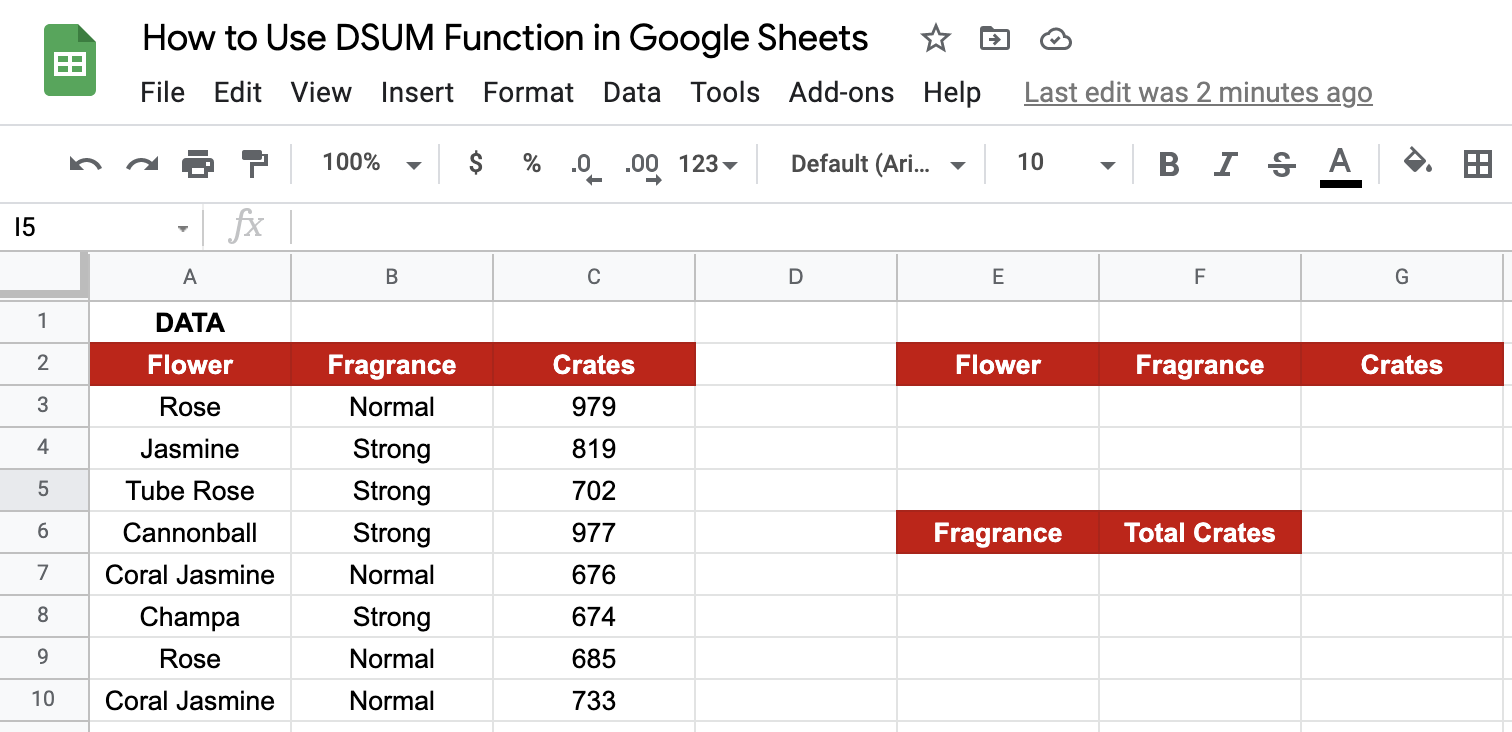
The above figures represent the total number of crates with a flower seller distinguished by the type of the flower – ones with normal fragrance and the ones with a strong fragrance. The objective here is to find the total number of crates of flowers with normal fragrance and crates greater than 500.
Just beside the captured data, I have given a provision to enter the criteria based on which the data will be filtered. This is not a required criterion, and the function will still function properly if we leave it blank. On applying the DSUM function on cell F7 after giving the required criteria under E3:G3, we will get the desired output as shown below

You may try changing the criteria and see how the result changes. Go ahead and make a copy of the spreadsheet using the link I have attached below:
Awesome! Let’s begin our DSUM() function in Google Sheets.
How to Use DSUM Function in Google Sheets
- Let’s see how to write your own
DSUM()function, step-by-step. First and foremost, I have listed the nutritional information for ten different types of biscuits that I consume throughout the day, from morning to night. I want to study the nutritional content I have consumed on a given day across all the variants.

I’ve made a list of the cases for which I’d like to find solutions and will try to get the desired outputs using the DSUM function
- Now, simply click on any cell to make it the active cell. For this guide, I will be selecting E19, where I want to show my results.
- Next, simply type the equal sign ‘=‘ to begin the function and then followed by the name of the function, which is our ‘dsum‘ (or DSUM, whichever works).
- You should find that the auto-suggest box appears with our function of interest. Continue by entering the first opening bracket ‘(‘. If you get a huge box with text in it, simply hit the arrow in the top-right hand corner of the box to minimize it. You should now see it as follows:
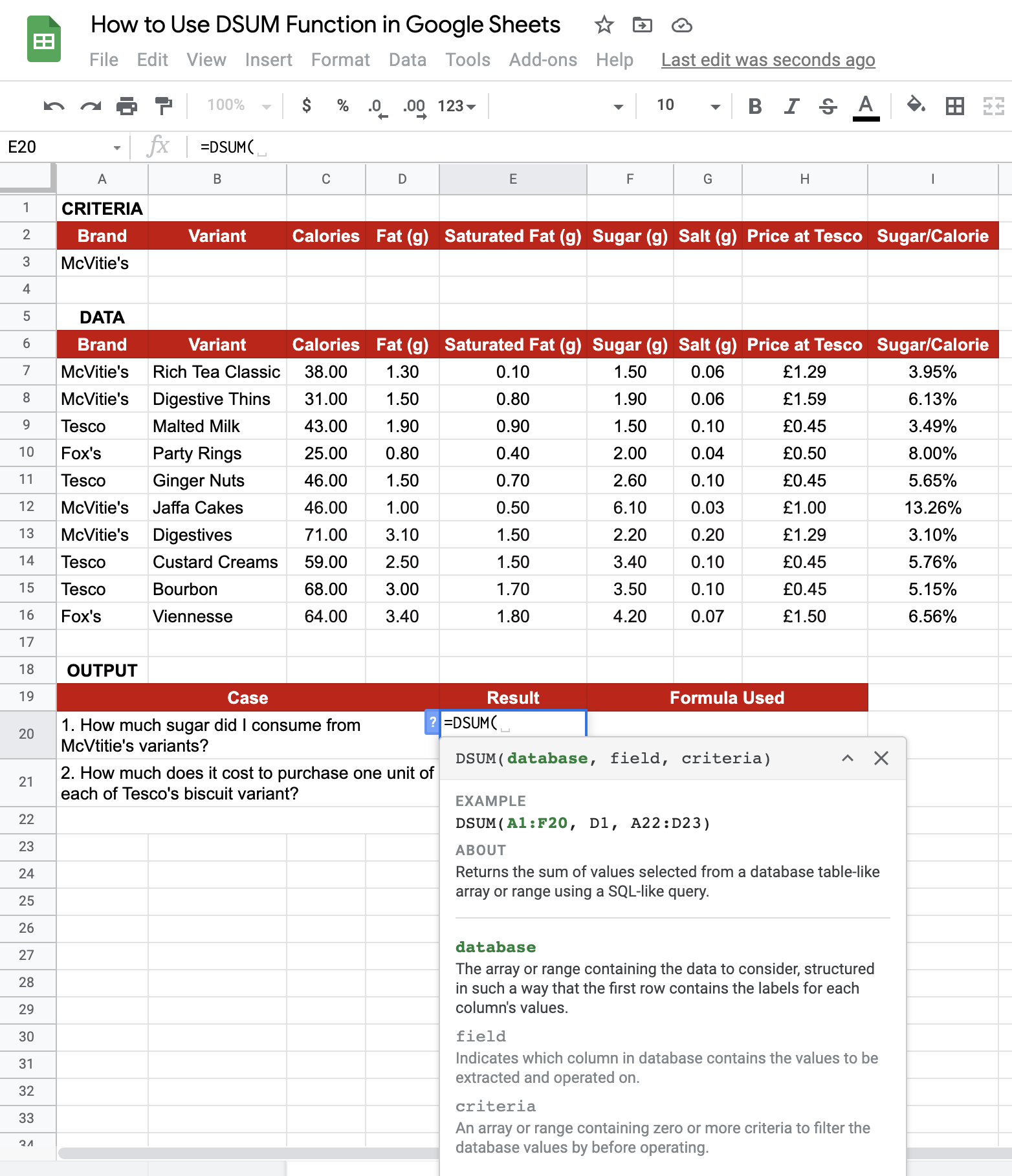
- Now, the fun begins! Let’s give the required inputs to the function to get the total sugar content from McVitie’s biscuit variants, per the filtration criteria we have given above the data:

- Take note of how I’ve specified conditions to limit the data to the Nike brand (selecting only the years 2019 and 2020). The criteria for the formula are input as A2:I9 to account for all the criteria mentioned, if any.
- Once you’ve entered the necessary database, field, and criterion values, or done what I did, close the brackets ‘)’, as shown below.

- Finally, just hit your Enter key. If you followed my instructions, you should have gotten 11.70 as the function’s output, which is nothing more than the variance of Nike and Puma combined unit sales (for the criteria specified above the data table).

9. Let us try one more case. This time, I am trying to find out the total cost required to buy one each of Tesco’s biscuit variants. If you apply the function similarly as above, you should be getting the below output:

Notice that the earlier result (for case 1) has been updated automatically to reflect total sugar content across the Tesco variants now, since you modified the criteria in A2:I3.
That’s pretty much it. You have everything you need to get started with the DVAR function on Google Sheets. I recommend experimenting with the DSUM function, combining it with the numerous Google Sheets formulas available, and seeing what you can come up with. 🙂