The COUNTIF function in Google Sheets is useful if you want to count the number of times a specific data is found in a selected range of cells that meets a single, specified condition.
Table of Contents
The COUNTIF function does this by combining both the IF Function and COUNT Function in your Google Sheets.
To break it down into its two components:
IF portion of the function determines whether the data meets a certain condition which results in either true or false. COUNT portion of the function totals up all the number of cells that meets the specified condition which is evaluated in our IF portion of the function.
Let’s take an example.
Say we have 8 pets (a mixture of cats and dogs). 🐱 🐶
We want to check the number of cats and the number of dogs that there are out of those 8 pets that we have.
So how do we do that?
Simple. We can use our COUNTIF function to enter the range of the pets that we want to test where the range would be our 8 individual pets.
We can then supply the function with the condition that we want to check which will be whether they are dogs "=dogs" or whether they are cats "=cats".
Finally, the function will output the number of cats or the number of dogs that there are amongst our 8 pets.
That’s all really how the COUNTIF function works. It’s simple and perfectly models our decision-making/counting process.
You can do a lot of things with this COUNTIF function as it is extremely useful for a whole variety of things.
Using the earlier example of our 8 pets, we can use our COUNTIF function to find out how many of those pets have the name "Jimmy". We can also use the function to test those 8 pets to see how many of those pets are younger than 5 years old "<=5".
See how easy that is?
It is one of the many powerful tools to have in your Sheetaki arsenal to solve a lot of your business data entry problems and shave half of your data entry time.
Let’s dive right into real-business examples where we will deal with actual values and textual strings and how we can write our own COUNTIF function in Google Sheets to compute those data.
The Anatomy of the COUNTIF Function.
So the syntax (the way we write) the COUNTIF function is as follows:
=COUNTIF(range, criterion)
Let’s dissect this thing and understand what each of these terms means:
- = the equal sign is just how we start any function in Google Sheets.
- COUNTIF() this is our
COUNTIFfunction. We will have to add our range and our criterion into it for it to work. - range is the group of cells that the function is to search.
- criterion is the condition where each cell in the range is to be tested whether it is to be true or false.
⚠️ Now a few notes when your range argument(s) contains numbers.
- You can use a comparison operator like > (greater than), <= (less than or equal to) or <> (not equal to) in your criterion expression. Each cell within the range will be checked to see if it meets the criterion.
- You do not have to use an equal sign ‘=‘ when you want to search for equal values. The value does not need to even be enclosed in quotation marks either. For example, the number 10 can be used as the criterion argument instead of having to write “=10” although both do work.
- You need to use double quotation marks when you’re planning to use non-equal expressions that do not include cell references. For example, “<=100”
- You should not enclose cell references in double quotation marks when you’re planning to use both comparison operators and cell references. For example, “<>”&A8 or “<=“&C3.
- You need to use an ampersand ‘&’ when you want to join the comparison operator with the cell reference. For example, “<>”&B2 or “<=“&C3.
⚠️ Now a few notes when your range argument(s) contains text data.
- You need to enclose text strings in double quotation marks. For example, “popcorn”
you can add wildcard characters like ? and * into text strings to match one (?) or multiple (*) contiguous characters. - You need to use a tilde ~ when you want to match an actual ? or a full-stop ‘.‘ For example, ~? , ~.
Now it may look like there’s a lot to know especially with everything noted above. Rest assured we will go through it and subsequently practice applying it. 🙂
A Real Example of Using COUNTIF Function
Take a look at the example below to see how COUNTIF functions are used in Google Sheets.

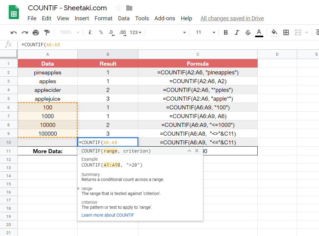
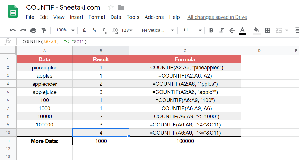
As you can see in the image above, the COUNTIF function to find the text “apple” in our data is found to have 4 results. The function is as follows:
=COUNTIF(A2:A6,"apple*")
Here’s what this example does:
- We have actively selected the cell (or box) under B6 (B column, 6th row) and we want to use the COUNTIF function to count the number of times the word “apple” is found in our data which is needed to be inserted into B6 as our result.
- We select rows from A2 to A6 as our range of data.
- We evaluate the range of data to count the number of times the word “apple” is found to be in the range of data which results in 4 times. We do this by making our criterion as “apples*“.
- Notice we use the * symbol to show the contiguous characters. This is because there is more than one case where the word “apple” is accompanied by other characters in the words within the data range like apple-“cider“, apple-“juice” and apple-“fruit“.
- As you can see the value ‘4‘ was inserted into our selected B6 because the term “apple” is found 4 times in our data — “apples“, “applecider“, “applejuice” and “applefruit” all have the word “apple” in them.
Easy peasy.
You may make a copy of the spreadsheet using the link I have attached below:
Let’s begin writing our own COUNTIF function in Google Sheets.
How to Use COUNTIF Function in Google Sheets
- Simply click on any cell to make it the active cell. For this guide, I will be selecting B10 where I want to show my result.

- Next, simply type the equal sign ‘=‘ to begin the function and then followed by the name of the function which is our ‘countif‘ (or ‘COUNTIF‘, whichever works).
- Great! Now you should find that the auto-suggest box will pop-up with the names of the functions that all show COUNTIF. The one we want is our COUNTIF function. So make sure to click on the right one! If you get a huge box with text in it (like below), simply hit the arrow on the top right-hand corner of the box to minimize it. You should now see as follows:

- Now what you need to do is select the range of cells that you want to use the COUNTIF function on. I will be highlighting cells A7 to A9 to include them as the function’s range argument.
- Next, we need to complete our function do that we can properly work. Enter a comma ‘,’ to act as a separator between our range and our criterion.
- Added the comma? Good. Now type the condition (expression) that you want to evaluate your data for. In this case, I want to test the data in my range whether they are lesser or equal to my value in cell C11, “<=”&C11. This will be the criterion.
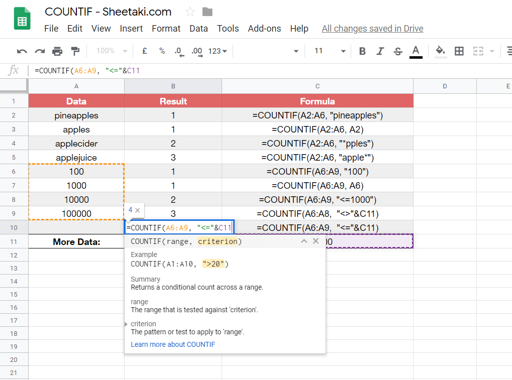
- Finally, just close the function with the closing bracket ‘)‘ then hit your Enter key. You’ll find that, if you followed my steps, that the result value in our B11 will be ‘4’. This is because all four of the cells in the range contain numbers that are less than or equal to 100,000.
That’s pretty much it. You can now use the COUNTIF functions together with the other numerous Google Sheets formulas to create even more powerful formulas that can make your life much easier. 🙂