The MONTH function in Google Sheets is useful to return the value of the month from any given unit of time, in numeric format.
Table of Contents
Although it is a simple date function, it can come handy if you are working with dates, but only care about the months. The MONTH function helps you remove the excess parts of those dates.
Let’s take an example.
Say you have a list of students with their birthdays and want to know who has a birthday this month. You will need to extract the month from the birthday.
So how do we do that?
Simple. The MONTH function just needs the date, and it will automatically return the value of the month in numeric format.
Let’s take a look at the anatomy of the MONTH function, to help you understand how to use it in Google Sheets.
The Anatomy of the MONTH Function
The syntax (the way we write) the MONTH function is especially simple, and it is as follows:
=MONTH(date)
Let’s break this down to help you understand the syntax of the MONTH function and what each of these terms means:
=the equal sign is how we begin any function in Google Sheets.MONTH()this is our function.dateis the unit of time from which to extract the month.
⚠️ A few notes you should know when writing your own MONTH function in Google Sheets:
- The
MONTHfunction cannot read all human-readable dates. As the input value, you will have to use either a reference to a cell containing a date, a function which returns a date object such asNOW,TODAYorDATE, or a date serial number of the type returned by the N function. - Be careful when using words in your dates, since the
MONTHfunction might return the error (#VALUE!). This happens if the date entered is not recognised as a number but as a text.
A Real Example of Using the MONTH Function
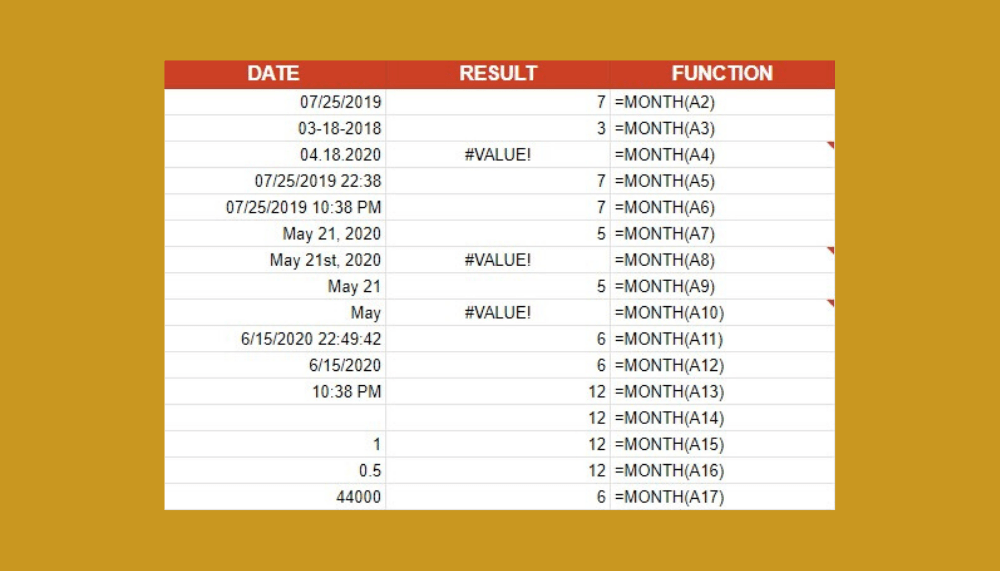
Let’s take a look at different date values and how will the MONTH function work with them.

The first two dates, in cells A2 and A3, are quite simple. The first one is written using slashes, while the second one is written using dashes. As we can see in column B, the MONTH function returned the value of the month in numeric format. However, in the next row, the MONTH function returned the error (#VALUE!) because the input value (cell A4) is not recognised as a date by our function.
In the next two rows, we used the same date as in the cell A2, we had just added time (cells A5 and A6). The MONTH function is still able to return the value of the month.
Now, let’s take a look at the next four rows, and what happens if use letters to write the name of the month (cells A7, A8, A9, A10). Two of them are recognised as dates (cell A7 and A9). Even though there is no year in the cell A9, the MONTH function returned the value of the month. However, if we write only the month (cell A10), with no year and date, the MONTH function will return the error (#VALUE!). The same goes if we write the day as ’21st’ (cell A8) instead of ’21’.
Date in the cell A11 is entered with the NOW function, while the date in the cell A12 is entered with the TODAY function. Both inputs are recognised as dates by the MONTH function. Note that these two values will change, and once you make a copy of the example spreadsheet, they will look different than in the picture above.
The ‘zero’ date
But what about the cell A13? This one is intriguing since there is no actual date but the MONTH function did return the value of the month. How is that possible? Simple. When there is no date but only time, the MONTH function will use the ‘zero’ date, which is 12/30/1899. The next row is similar. If the cell is blank (cell A14), the MONTH function will use the ‘zero’ date, as well.
If we input a random number into a cell (cell A15) and use the MONTH function, the ‘zero’ date will be incremented by that number (12/30/1899+1=12/31/1899). Even though we are not able to see that, if we input only a decimal with no whole numbers, the ‘zero’ date will stay the same, only hours, minutes and seconds will be incremented.
To get to the present date, you should enter 44000 (cell A17). The MONTH function will return ‘6’ since the whole date (the ‘zero’ date incremented by 44000) is 06/18/2020.
How to Use the MONTH Function in Google Sheets
Let’s start writing our own MONTH function in Google Sheets, so you can take a look at how it works and what should you pay attention to.
- First, click on a cell where you will write the
MONTHfunction, to make it active. For this guide, I will use the cell C2.

- Type the equals sign ‘=’ we use to begin any function, and start typing the name of the function, which is ‘MONTH’. As you start typing, the auto-suggested box with the names of the functions that start with the same letters will pop-up. You can just continue typing or you can select the
MONTHfunction from the list.

- Enter the opening round bracket ‘(‘ and input the date the
MONTHfunction will return the value of the month from. Since we have our date in column B, we will use the cell reference instead of typing the date into theMONTHformula. Enter the B2 and close the function with a closing round bracket ‘)’ or by pressing the Enter key on your keyboard.

- If you did everything right, the
MONTHfunction will return ‘8’. Now repeat these steps for all other students.

That’s it! You did it! Now you know who has a birthday in June and you have learned how to use the MONTH function in Google Sheets. You can make a copy of the spreadsheet using the link below and try it for yourself:
You can also use the MONTH function together with the other Google Sheets formulas to create even more effective formulas that will save you time and help with your data 🙂