The ABS function in Google Sheets returns the absolute value of an integer. It converts negative numbers to positive numbers.
The ABS function in Google Sheets has three straightforward methods that you can use.
Table of Contents
The rules for ABS function in is defined as follows:
- There is only one argument in ABS function
- ABS function does not affect numbers with 0 value
Here’s a sample scenario.
Joseph wants to know how to return the negative value of a number in Google Sheet to its absolute form. Joseph does not want to put simply a negative sign on the right of the number because he believes that it might cause some errors in the data. Using the ABS function in the Google Sheet, Joseph pulls up the following:
Here’s how Joseph did it. But first, let us learn the important details of the ABS Function.
The Anatomy of the ABS Function in Google Sheets
The syntax (the way we write) of the ABS function is as follows:
Let us dissect the function and understand what each of these terms means:
- = the equal sign is just how we start any function in Google Sheets.
- ABS () is our ABS function in Google Sheets.
- Value refers to the number that will be converted to an absolute value
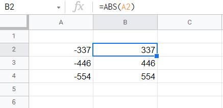
A Real Example of ABS function in Google Sheet
Let us check the data below and see how the ABS Function works.
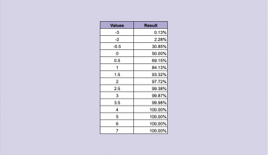
By default, several functions in Google Sheets will return negative numbers. The majority of them are associated with the monetary outflow.
Let us look at the PMT function in Sheets as an example. This is a financial function that assists us in calculating the loan payment.
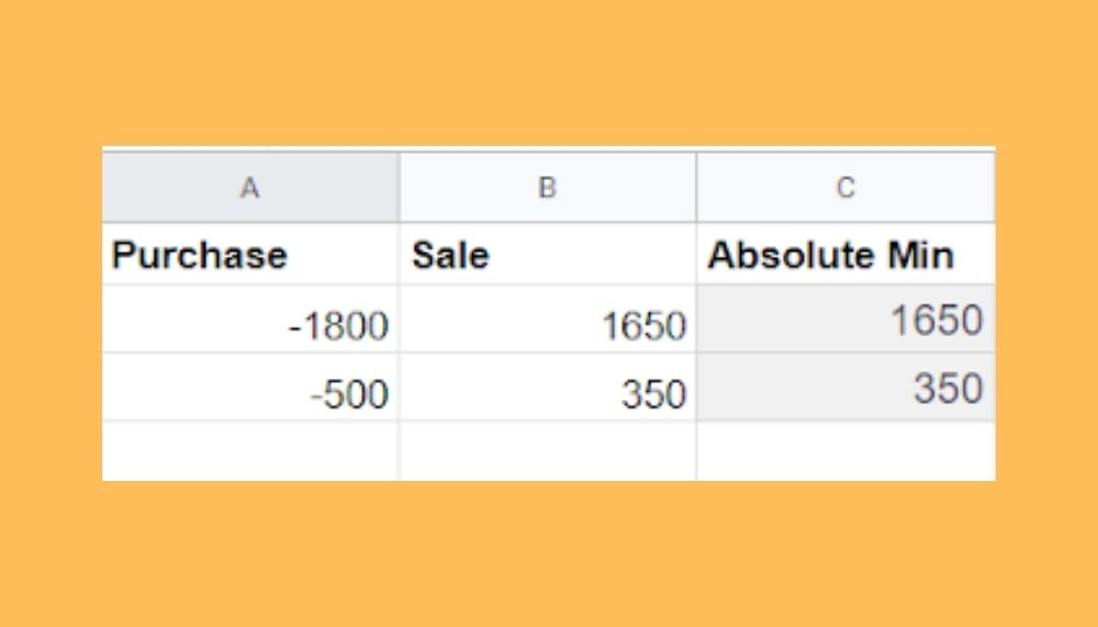
Min or Max Ignoring the Sign of the Numbers
Use the following formula if you wish to get the Min or Max of two numbers while ignoring their sign.
Data Sample:
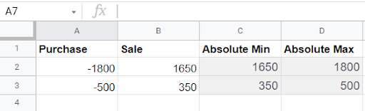
Because the purchase represents a monetary outflow, such transactions are recorded as negative values. When entering such data, we may utilize the ABS function with MIN/MAX methods to get the minimum or maximum value regardless of the sign.
C2’s Min Formula states that the purchase value is smaller than the sales value (Absolute MIN).
In C3, the minimum formula states that the sales value is less than the purchase value (Absolute MIN).
In D2, the Max Formula states that the sales value is larger than the purchase value (Absolute Max).
The purchase value is more than the sales value, according to the Max Formula in D3 (Absolute Max).
Let’s learn together. Click on the link below and make a copy of the spreadsheet that we are using.
Now, let us, deep-dive, into the step-by-step guide.
How to Find ABS Function Absolute Value in Google Sheets?
In Google Sheets, finding the ABS function’s absolute values is as simple as using one of three methods: the ABS function, the SUMPRODUCT function, or turning negative integers into positives.
Please take a look at the three (3) approaches listed below to learn how to utilize them.
- Open the spreadsheet in Sheets. Select the Add-ons option from the pull-down menu.
2. Then select Power Tools.
3. To access Power Tools, select Start from the pull-down menu, as seen in the picture below.

4. From the option that appears on the right, select Convert.

5. Tick the Convert number sign checkbox.

6. Select Convert negative numbers to positive from the drop-down menu.

7. With the cursor, choose the cell range A2:A4 on your Sheets spreadsheet.

8. In the add-ons sidebar, click the Run button.

As illustrated in the picture below, this method eliminates the negative indications from cells A2:A4. Absolute values have replaced negative values in some cells. With this conversion option, we may quickly obtain the absolute values for a large number of cells without having to put any ABS functions in a neighboring column. The Power Tools Add-on has quickly become a must-have for Google Sheets power users.
Frequently Asked Questions (FAQ)
1. What is the importance of using the ABS function?
We could always manually convert negative values to positive ones if we only wanted to acquire a single or two cells’ absolute value. Consider a vast spreadsheet with a table column containing 350 negative values.
2. Why is Google Sheet’s ABS function much better to use than any other spreadsheet?
The ABS function allows us to rapidly obtain absolute values for negative integers without altering their cells. It is a simple function that we may enter using the following syntax: =ABS (value). ABS values can be either cell references or numbers.
3. How do you do absolute value on a spreadsheet?
It is a simple function that may be entered using the following syntax: =ABS(value). ABS values can be either a cell reference or a number or anything inside a cell that has values.
How was your experience learning and practicing ABS function in Google Sheets? Take note of what you have learned, as you can use this in the near future. That is for today’s how-to guide. You may also check this article for some Google Sheet tricks.
Do not forget to subscribe to our newsletter for more informational articles like this.