The WORKDAY.INTL function in Google Sheets is useful if you want to get a date that is the N working days in the future or the past with an option to determine days that would be weekends.
Meaning, the WORKDAY.INTL function returns a date that is either after or before a certain number of days from the provided start date and allows us to customize which days of the week are considered weekends.
Table of Contents
The rules for using the WORKDAY.INTL function in Google Sheets are as follows:
- The function will return the #NUM error when the arguments provided result in an invalid date or any of the provided holidays is invalid.
- If the provided second argument, which is the days, is not an integer, it will be truncated.
- The function will return the #VALUE error when the dates arguments are not valid dates and the days provided are non-numeric.
- Furthermore, the function will return the #VALUE error when the provided weekend argument is invalid.
- It is recommended that for the dates arguments, they should be entered as either reference to cells containing dates or dates returned from formulas.
Let’s take an example.
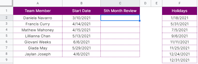
Fletcher manages a team of seven in a BPO company and was asked to create a roster that shows each team member’s start date and 5th-month review date. In his company, the 5th-month review is being given to a team member on the 110th working day excluding US holidays.
See his created roster in Google Sheets below:

Unfortunately, he can’t use the WORKDAY function in this scenario, which considers Saturday and Sunday as the default weekends, since his team is on time off during Mondays and Tuesdays.
So, he needs a function that’s as good as WORKDAY.
That’s where our WORKDAY.INTL function will come in handy. It’s the modification of the WORKDAY function, as it has an option to change the weekends.
Fletcher used the WORKDAY.INTL function and it’s exactly the function he needs to get the 5th-month review date of his team members.

Pretty convenient, right?
Watch out for a more advanced tutorial and examples on how you can use the WORKDAY.INTL function in the coming weeks. Be sure to subscribe to be notified.
Perfect! Let’s begin getting to know more about our WORKDAY.INTL function in Google Sheets.
The Anatomy of the WORKDAY.INTL Function
So the syntax (the way we write) of the WORKDAY.INTL function is as follows:
=WORKDAY.INTL(start_date, days, [weekend], [holidays])
Let’s dissect this thing and understand what each of these terms means:
- = the equal sign is just how we start any function in Google Sheets. It is how Google Sheets understand that we are asking it to either do computation or use a function.
- WORKDAY.INTL() this is our WORKDAY.INTL function. It returns a date N working days in the future or past with an option to specify which days of the week are the weekends.
- start_date is the date from which to start.
- days is the number of workdays to be added to start_date. If we enter a positive value, it will give us a future date, while a negative value will yield a past date.
- [weekend] is an optional argument. A value that would set which days of the week should be considered weekends.
- [holidays] is an optional argument. This is the list of dates that should be considered non-work days.
A Real Example of Using WORKDAY.INTL Function
Let’s take a look at the roster that Fletcher created below to see how the WORKDAY.INTL function is used in Google Sheets.
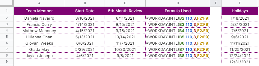
Fletcher was able to yield his team member’s 5th-month review date or their 110th working day since the start date using the WORKDAY.INTL function.
The dates in column C are 110 days from the start dates in column B. This excludes US holidays, which were listed in column F.
The WORKDAY.INTL function also considers that the team’s rest days fall every Monday and Tuesday.
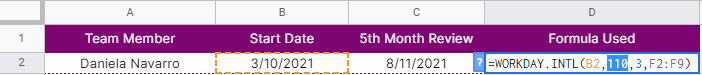
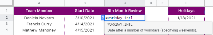
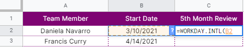
Let’s take a look at the example in the second row. He just passed four arguments to our function. The first one is the start_date, which tells the WORKDAY.INTL function where to begin counting. In this case, it is the start date of each team member.

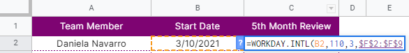
The second argument is integer 110, which tells the WORKDAY.INTL function the number of working days it needs to add from the start_date.
Now, unlike the WORKDAY function, the WORKDAY.INTL function allowed Fletcher to change the default weekends into different days of the week. In this case, Mondays and Tuesdays were used as weekends instead.
How did Fletcher do that?
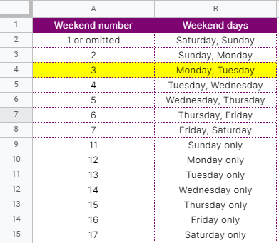
Simple. He passed integer 3, which means weekends are Monday and Tuesday, as the third argument in the WORKDAY.INTL. You may refer to the list of values below with their corresponding weekend days:
Alternatively, Fletcher could have passed the string ‘1100000’ instead. This corresponds to Monday and Tuesday as weekends as well.
The third argument can be a string value, which is a series of seven 0’s and 1’s that represents seven days of the week, beginning with Monday. 1 represents a non-working day and 0 represents a workday. For example:
“1000001” – Monday and Sunday are weekends.
“1100000” – Monday and Tuesday are weekends.
Lastly, the third argument is an optional list of US holidays that Fletcher didn’t want the WORKDAY.INTL function to include in counting.

In this case, he put all the US holidays for the year 2021 in column F from the second row until the 9th row.
The return value of the WORKDAY.INTL function in our example above is the date ‘8/11/2021. This means that it’s the 110th day from the start date ‘3/10/2021’ treating Mondays and Tuesdays as weekends and excluding US holidays.

Like the WORKDAY function, you can pass a negative integer to the second argument of the WORKDAY.INTL function to move back.

You may make a copy of the spreadsheet using the link I have attached below.
How to Use WORKDAY.INTL Function in Google Sheets
- Click on any cell to make it the active cell. For this guide, I will be selecting C2, where I want to show the result.
- Next, type the equal sign ‘=‘ to begin the function and then follow it with the name of the function, which is our ‘workday.intl‘ (or ‘WORKDAY.INTL‘, not case sensitive like our other functions).
- Type open parenthesis ‘(‘ or simply hit Tab key to let you use that function.

- Now the exciting part! Let’s give our function its only argument, the start_date. Click the cell where our order date is located. In this case, click on cell B2. Alternatively, you may type in ‘B2’.
- To let the Google sheet know that we’re done typing our first argument, we should now type in the delimiter or the character that separates each argument on a function. In this case, type comma ‘,’.

- Type in our second argument, which is the days. In this case, we will use ‘110’ to denote 110 working days. Type in ‘110’ and follow it with another comma ‘,’.

- Pass the third optional argument, which is the [weekends]. Since we need to tell the WORKDAY.INTL function to take Mondays and Tuesdays as the weekends, we will use ‘3’. Type in ‘3’ and follow it with a comma ‘,’.

- Now, provide the last but another optional argument, which is the [holidays]. Since we put the list of US holidays in range F2:F9, type in ‘$F$2:$F$9’. The dollar ‘$’ character means we are making the range an absolute reference since we are copying the formula down to the remaining rows later.
- Finally, hit your Enter or Tab key. Cell C2 will now show you the return value of the WORKDAY.INTL function, or the 110th working day from the start date provided.

- Copy the formula down to cells C3 to C8.

That’s pretty much it. You can now use the WORKDAY.INTL function in Google Sheets together with the other numerous Google Sheets formulas to create even more powerful formulas that can make your life much easier.