How to Use SUMX2PY2 Function in Google Sheets

The SUMX2PY2 function in Google Sheets is a mathematical function designed specifically to calculate the sum of the squares of each number in two arrays.

In other words, this function returns the sum of the sum of squares of corresponding values in two arrays. 

The sum of the sum of squares is a common term in many statistical calculations.

So, what’s an array?

An array in Google Sheets is a series of populated cells, whether horizontal or vertical. Meaning, either one row of cells or one column of cells.

Now, consider that we have an array named ‘A’ with the following three numbers (2, 3, and 4), and an array named ‘B’ with these numbers (3, 5, and 4). Now, if we want the sum of the sum of squares of these two arrays, we use the SUMX2PY2 function.

So, what would be the calculation equation for the previous example? Let’s see.

Here’s the general equation for the sum of the sum of squares:

Now, if you apply this formula to our data for arrays ‘A’ and ‘B’, we get the following equation:

Sum of the sum of squares = (2² + 3² + 4²) + (3² + 5² + 4²) = 79

Alright I’m sure the SUMX2PY2 function is a bit clearer now, but let’s go ahead and learn more about it in the next section.

The Anatomy of the SUMX2PY2 Function in Google Sheets

 So, the SUMX2PY2 function shall be written as follows:

= SUMX2PY2 (array_x, array_y)

Let’s dissect this thing and understand what each of these terms means:

• = (the equal sign) is just how we start any function in Google Sheets.
• SUMX2PY2 is the name of the function we are using.
• () These parentheses are used to host the two values we put in our function, and a comma “,” must separate these values.

Note that the values hosted in any google sheets function are called arguments.

• (array_x) 1st argument. This argument takes a series of cells in either one row or one column.
• (array_y) 2nd argument. Same as the argument before.

Alright, let’s take a moment here before we dive deeper into this function. There are some things to be aware of. Or else, your results won’t be accurate.

• If any of the two arrays selected in the function contains a text format, this text will be considered with a value of 0.
• If there is a date in any of the arrays in the function, this date will be considered the date value, which may be a very large number, that will mess up your calculations.
• The two arrays you put into the SUMX2PY2 function must be of the same size, otherwise, an error will occur.

Now for further explanation, let’s go through the SUMX2PY2 function together, and you will understand it once you start practicing its application.

A Real Example of Using SUMX2PY2 Function

Take a look at the example below to see how the SUMX2PY2 function is used in Google Sheets.

Let’s say we have the two following arrays.

• Array X: 15, 12, 11, 4, 5, 8, 2, 6, 12, 21, 14, 89
• Array Y: 10, 9, 7, 6, 3, 2, 31, 8, 11, 4, 5, 19, 36

And that’s how we input our data into Google Sheets: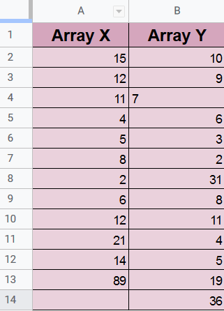

Alright, now tell me, at first glance do you notice anything that might cause a faulty result?

Well, it’s the value in cell B4, being left aligned like that should indicate that it’s of the text format, which means it will be equal to 0. So, it definitely needs fixing to avoid any mistakes.

Let’s see how to fix it in two steps:

1. First, let’s look at its current format.
2. Then we change its format from text to ‘Number’ or ‘Automatic’.
   You can see now that it’s fixed, as it became right aligned.

Alright, now that we have prepared our two arrays, let’s calculate their ‘sum of the sum of squares’ using the SUMX2PY2 Function of Google Sheets.

You may make a copy of the spreadsheet using the link attached below.

Make a copy of example spreadsheet

How to Use the SUMX2PY2 Function in Google Sheets

1. Simply click on any cell to make it the active cell. For this guide, I will be selecting C2, where I want to show my formula. Then type “=”.
2. Now, type “SUMX” and click on the SUMX2PY2 function, press the Down Arrow twice, and press Tab to select it.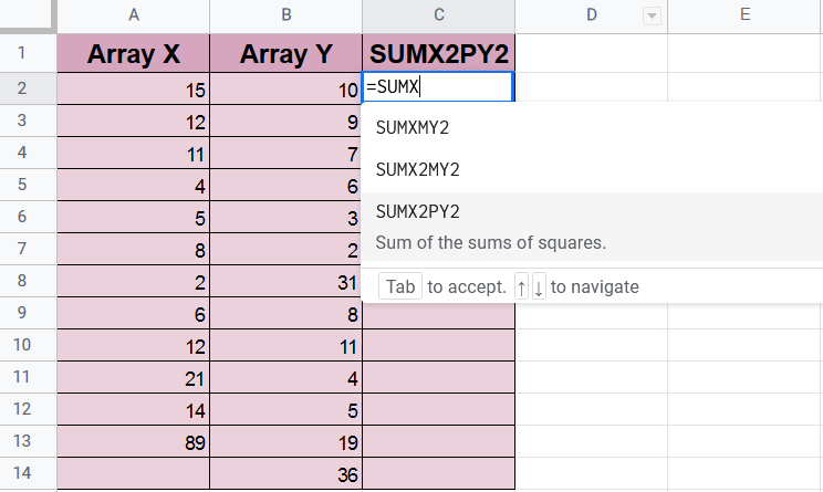
   Notice that there are three options to select from, we are only concerned with the SUMX2PY2 function now, so don’t confuse it with the other ones; SUMXMY2 and SUMX2MY2, as these functions are different.
3. Now, fill in the first argument of the function, array_x, which would be the range in cells A2:A13. So, you can select it or simply just write ‘A2:A13’.
4. Then, type comma “,”.
5. Now go ahead and select the second argument, array_y, which is the value in B2:B14.
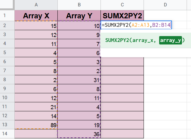
6. Now, close the parenthesis, press Enter, and let’s see what happens.
7. Oops! We get an error. After reading the error, we realize that both arrays selected must be of the same range. Well, that’s an easy fix. We just need to re-select our first argument to be A2:A14.
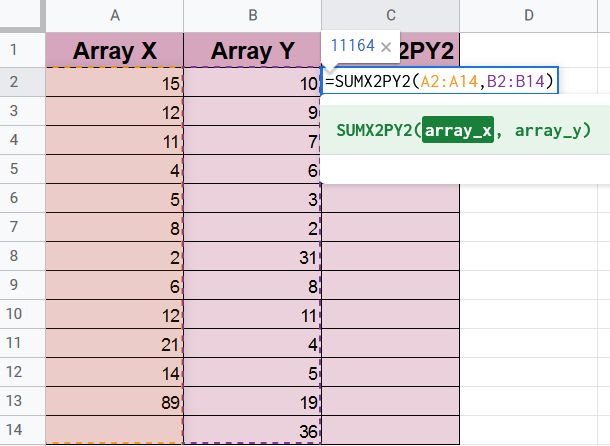
   You see now that our result (11164) is ready to display, even though cell A14 is empty, which means it’s valued as 0, which we initially intended.
8. Finally, press Enter, and the correct result will take over.

That’s pretty much it. Congrats! You now learned the SUMX2PY2 function in Google Sheets.

Are you looking forward to learning some more amazing Google Sheets Functions? Well, you are in luck, as you are a single click away from your destination.

Get emails from us about Google Sheets.

Subscribe