Very often than not, we would face some trouble with formulas in Google Sheets. A common error that appears while using the FILTER function is the mismatched range sizes error. Usually, the mismatched range sizes error comes up when the filter values you inputted into the formula do not have the same number of columns or rows.
Do not worry! We will be learning different ways to identify what may be the cause of this error and how to fix it! 🤗
Here are some of the main causes for this error to appear:
- Inputting different ranges of data
- Forgetting to input the sheet name
For those who are not familiar with the FILTER function, don’t be shy, and go over to our tutorial for a more in-depth demonstration before proceeding to the rest of this tutorial!
Table of Contents
Filter Has Mismatched Range Sizes Error Due to Inputting Different Ranges of Data
Several scenarios cause the FILTER function to show a mismatched range sizes error in Google Sheets by inputting different data ranges into the formula. Some common scenarios are:
- Input not starting or ending at the same row (for data filtered vertically)
- Input not starting or ending at the same column (for data filtered horizontally)
Let’s use some examples to give you a better visualization and how to solve such errors.
Example 1:
For this example, we will be using a data set containing the profit achieved by different businesses located in different states. To organize each state’s profits, we would use the FILTER function to make this happen.
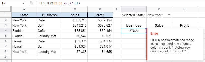
However, the formula returned with a filter has a mismatched range sizes error. Let’s see how we can fix it.
One of the common errors in the formula would be the inputs not starting or ending at the same row.
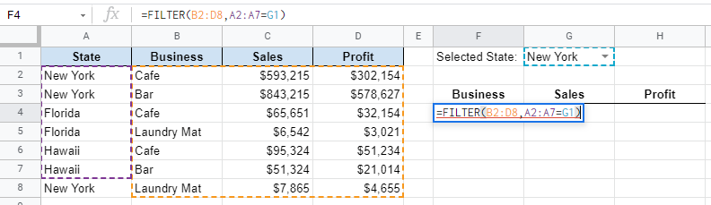
We can see that the condition attribute that is inputted does not match the range attribute. To fix the error, we should match the condition attribute to the range attribute by ending at the same row, which is row 8.
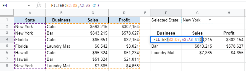
So the formula should be:
=FILTER(B2:D8,A2:A8=G1)
Example 2:
A mismatched range sizes error can also occur when the input does not start at the same row.

Similar to Example 1, the condition attribute does not match the range attribute as it does not start on the same row.
We can simply amend the condition attribute to start on from row 2.
This would result in the same formula as Example 1.
Example 3:
What if your data are displayed you need to filter horizontally? The same rules apply. The conditional attribute and range attribute inputs must match.

Instead of starting or ending at the same row, it needs to start or end at the column.
As we can see in the example, the condition attribute should start from B1 instead of C1.

After matching the inputs, our formula should look like this:
=FILTER(B2:H4,B1:H1=B6)
Filter Has Mismatched Range Sizes Error Due to Forgetting to Input the Sheet Name
Another common reason the filter has a mismatched range sizes error is forgetting to input the sheet name.
When we use the FILTER function to filter data deriving from another sheet, we must specify the sheet name.
Example 1:


You can see in this example, the data used in the FILTER function is taken from another sheet.
To resolve this error, we would need to specify the sheet name that the data for the condition attribute is deriving from.
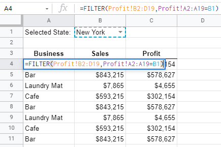
Simply add in the sheet name and the FILTER function will work just fine!
Don’t forget that the previous rules still apply. The inputs must start and end at the same row or column.
That’s it! Follow these two simple rules, and we guarantee that your FILTER function would work every time! 🤸♀️
You may make a copy of the spreadsheet using the link attached below and try it for yourself: