The DMAX function in Google Sheets is useful if you want to find the maximum value in a database based on the given criteria.
In this guide, you will learn how the function is derived and how it is used in real-life situations. Also, we will provide you with visuals for a clearer understanding of the DMAX or otherwise known as the database maximum function.
Table of Contents
The DMAX function is helpful especially when you are dealing with hundreds and thousands of information in one database.
Imagine that you are running a chain of hotels and you have 600 employees in total. You want to find out who among these employees has the biggest salary loan. If you have all the names and values in a single database, the DMAX function will make the work easier.
An additional example would be if you have thousands of students in your school and you need to look out for the student who has the highest payable. Why not use the DMAX function to make it easier to look it up?
There are lots of other instances where this function is handy. Instead of spending your time on scrolling each and every column and row, the DMAX function will make things work quicker for you.
Let’s implement the first example in this entire DMAX function guide.
When you have to know how much the biggest salary loan is, by using the DMAXfunction, it will automatically output the greatest salary loan among 600 employees in just a second.
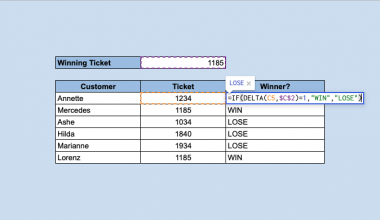
Using this scenario, we can also identify which among the salary loans is the oldest. By adding another column that we can name as “Years”, we can replace the previous criteria, ‘salary loan’ to ‘Years’.
Let’s now focus on how the DMAX function is used and applied in real life.
The Anatomy of the DMAX Function
Take a look at the example below to see how DMAX functions are used in Google Sheets.
=DMAX(database, field, criteria)
Let’s dissect this thing and understand what each of these terms means:
- = the equal sign is just how we start any function in Google Sheets.
- DMAX() this is our function. For it to be operational, we have to add 3 attributes, namely, the database, field, and criteria.
- database is the source of our data. It is the whole data itself, including the headers or names of headers.
- field is the header of the column or row where you want to get your data from.
- criteria is the array/range of cells containing the condition. It is the column or row of the field, including the field itself.
⚠️ Now a few notes before using the DMAX Function:
- You must separate each attribute with a comma ( , ) for your
DMAXfunction to work properly. - For the field section, you can simply click on the cell of the header. If you want to use another way, you can also type in the name of the header (label) and include ” ” (e.g. “Salary Loan”).
- In filling out the range/cells for the criteria section, do not forget to include the field itself.
Now it may look like there’s a lot to know especially with everything noted above. Rest assured we will go through it and subsequently practice applying it. 🙂
A Real Example of Using the DMAX Function
Take a look at the example below to see how DMAX functions are used in Google Sheets.


In this example, we are trying to find out the biggest salary loan among these chosen employees (A to E). The formula led us to an answer of $250.00.
Here’s a step-by-step guide on how we came up with $250.00:
- We wanted to find out the largest Salary Loan.
- Remember the syntax,
=DMAX(database, field, criteria). - For the database, we selected the entire data, including the headers. In our example, we selected cells
A1:E6. - Since we are trying to look out for the biggest salary loan, we clicked the ‘Salary Loan’ header,
D1. - For the criteria, we selected the entire ‘Salary Loan’ column including its header,
D1:D6. - Finally, adding all this together, we get the formula:
=DMAX(A1:E6, D1, D1:D6). Hit the Enter key and the formula gives us the $250.00 as a result. This is correct as Employee B has the largest ‘Salary Loan’.
Easy, right?
You may make a copy of the spreadsheet using the link I have attached below:
Try to begin writing a DMAX function in Google Sheets. For your practice, I added another column, “Age” which denotes how old the loan is. Can you work on your formula to get the oldest loan (Age)?
How to Use the DMAX Function in Google Sheets
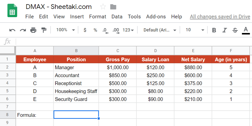
- Click on an empty cell to make it an active cell. In this guide, I chose B8, as shown below.
- Next, simply type in the equal sign “=” as the start of the syntax, followed by the name of the formula which is
DMAX. You can write it in lowercase or uppercase, depending on what works best for you.

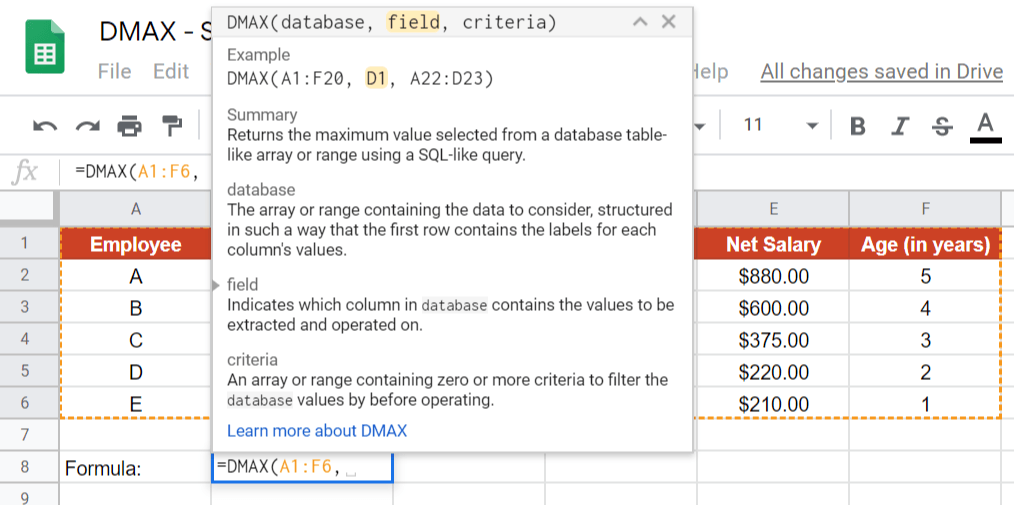
- Add an open parenthesis ‘(‘. The syntax will auto-populate along with a summary of the function and a short description of each attribute. This will serve as your guide to input the right attributes.

- First, we will add the database. To do this step, we will have to select the entire data (A1: F6).

- Good job! Next, before we start to input the field, we have to put a comma ( , ) after F6. The comma serves as a separator.
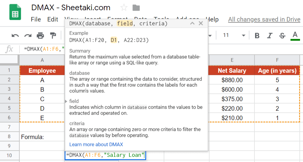
- Next, since we are looking for the biggest salary loan, then the field is the Salary Loan. We simply have to click on D1.

- Another way to do this is to spell out the name of the header and adding “ ”, as shown in B10.
- Get ready to move on to the next attribute of this
DMAXsyntax. Add a comma (,) after D1 (or after the end quote “, if you did the other way).
- Lastly, we will now input the criteria. To do this, you have to select the column (which you want to look for including its header, followed by a closing parenthesis. In this case, I’ve added D1:D6, which is the column for Salary Loan.

- Hit the Enter key to get the result. Voila!

And that’s it! Great job on that! You can now use the DMAX function together with the other numerous Google Sheets formulas to create even more powerful formulas that can make your life much easier. 🙂