How to Highlight Cells Based on Multiple Conditions in Google Sheets

A few days ago, my wife and I were organising our yearly budget for the family. 

I was tired of using templates from Pages, Microsoft Word, and other platforms. Precisely because editing those templates meant we would be impacting the design and therefore defeats the whole purpose of the template.

Then I decided it was time to learn how to build my own, and if you are also like me who avoided using those applications, then look no further. 

I wanted cells to highlight specific colours based on conditions. The conditions were whether we went above budget or below. Some of you who do data entry and need to keep track of things will understand the frustration of using pre-made templates but learning to do it on your own should never be so tedious and time-consuming.

Here is a step-by-step guide on how you can highlight cells based on multiple conditions in Google Sheets.

Highlighting a Single Cell.

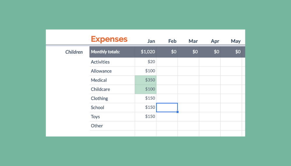
First of all, create your template for whatever data entry purpose you wish to use it. I wanted to be on top of my budget for the year and understand our family finances. So I have used the generic template that comes with Google Sheets for demonstration purposes.

Now I wanted for the Allowance tab to not go over $100, but if it did, I wanted to be highlighted.

So select the cell, and on the menu bar, select Format then click on Conditional formatting. 

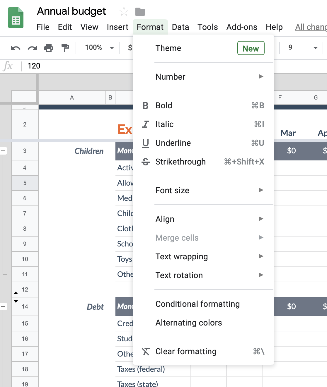
Once you have selected conditional formatting, you will see options on the right-hand side of the page to edit.

As you can see in the image below, there are several options available to you.

First is the range of cells  (Apply to range) you can select. I selected cell D5, which is the Allowances tab, and I also decided that I want the cell to be highlighted in the Default (Green) colour if the budget went above $100. You can change this colour to any colour which you may prefer.

Under Format rules, I selected the rule “Greater than” from the dropdown box and inserted the value of 100. This means, if a value in the range is greater than 100, then the cell is highlighted as green. You can see this in action below:

Highlighting Multiple Cells.

Let’s say I wanted to get on top of my debt. To do that I wanted to make sure I repay amounts monthly without missing a single payment. To make sure I know where I sit with my loan repayments I want the cells to highlight to red colour in case I do enter a value I have repaid.

This way, you can format multiple cells and select rules that you want to apply to them. It is done similarly to that of highlighting a single cell, but for this, you have to select multiple cells instead. In my case, I have chosen all cells within Debt Repayments. 

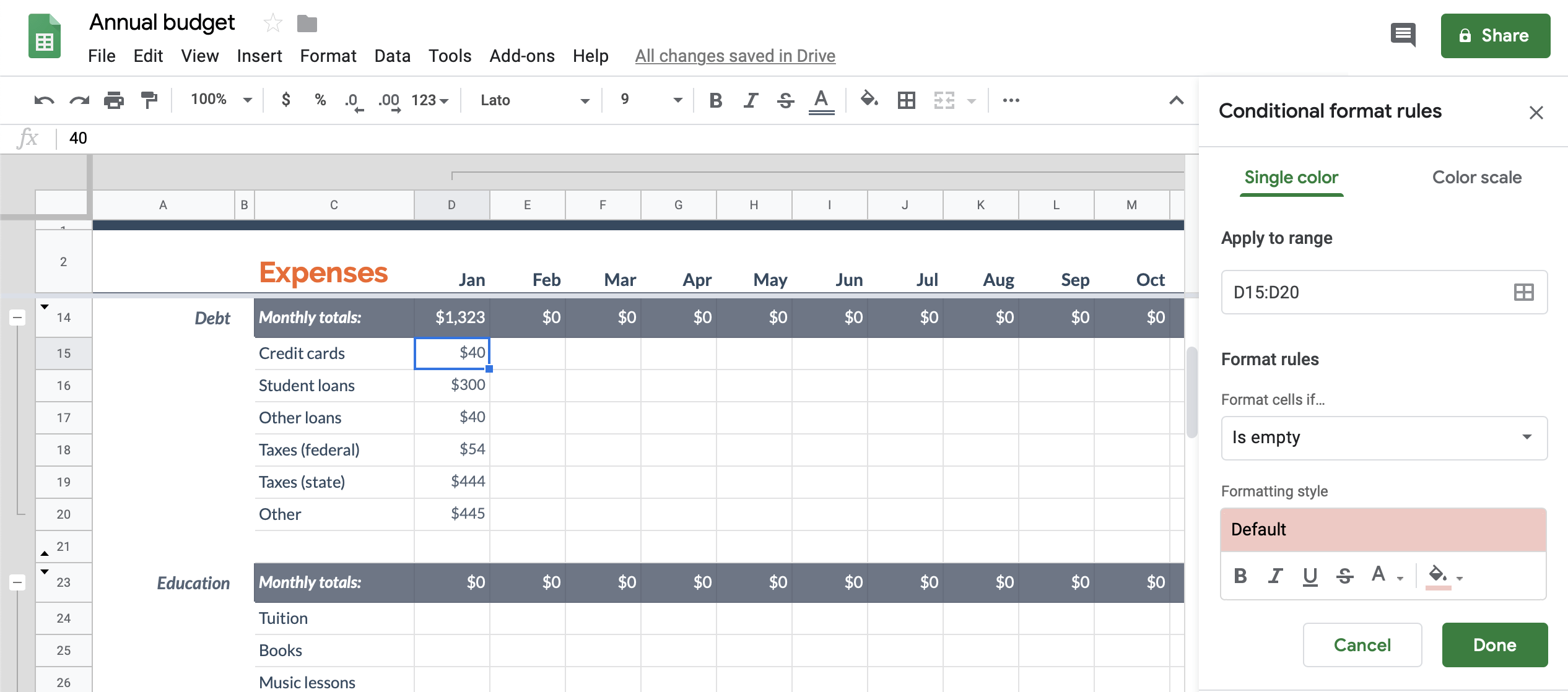
On the right-hand side of the below image, you can see that I have selected a range of cells (Apply to range) that were related to Debt and have chosen the rule to be Is empty (under Format cells if...) with the highlight colour as pink (Formatting style).

Now hypothetically, if I were to miss a payment on one of the loans, the cell would be highlighted.  

You can achieve the same outcome by formatting the cells using formulas but with the added benefit of better automation, and dynamism.  What you saw above is formatting cells without using formulas.

In most cases, you may need to take it further than conventional templates for rules and apply your own. In which case you can utilise functions such as IF, AND and OR that you’ve learned within Google Sheets. We provide a few examples below which you can try out. 🙂

As you can see from above, I have added the cell D7, and chosen Customer formula is (under the Format cells if...) as the option and have entered the following formula:

=AND(D7=100)

This formula means is that If Childcare expenses would reach 100, then the cell would be highlighted.

You can also add the OR function to spice things up — which works by basically looking at two statements and then proceeds to evaluate when if one of them is True, then all statements are True.

Look at the image below to see this in action: 

You can see I added cell D8 to the range and have combined the OR function with the formula:

=AND(OR(D7=100; D8=80))

What it means is that if one of the cell either equal 100 or 80, then both of them would be highlighted.

With this, you will be able to apply this technique to any range of multiple cells across the spreadsheet with any rule you seem fit for your spreadsheet. I encourage you to play around and unleash your creativity using and combining the various Google Sheets functions available.

I hope you have as much fun as I did learning how to highlight cells based on multiple conditions in Google Sheets. 🙂

Get emails from us about Google Sheets.

Our goal this year is to create lots of rich, bite-sized tutorials for Google Sheets users like you. If you liked this one, you'll love what we are working on! Readers receive ✨ early access ✨ to new content.

Subscribe