How to ROUND Numbers in Google Sheets

The ROUND function in Google Sheets is useful if you want to reduce a value by a specific number of decimal places.

Meaning, the rounding digit(s) is rounded up or round down to provide a more manageable figure.

The rules for rounding numbers in Google Sheets are as follows:

• the value of the number to the right of rounding digit is less than five, the rounding digit is left unchanged.
• If the value of the number to the right of the rounding digit is five or higher, then the rounding digit is raised by one.

Let’s take an example.

Just the other day I was trying to log my daily grocery expenses and you know how some products are priced like $12.90 or $17.95?

Well, dealing with decimal numbers is a nightmare when you’re keeping tabs on the total expenses when they have .96, .52, .01 values at the back. Hence, by using the ROUND function, I was able to round up to the nearest value to easily total up my expenses.

So for a packet of spaghetti, that costs $11.95, I was able to ROUND it up to $12.00 using the function whereas a jar of pesto which was $6.35 will be ROUND up to $6.40.

Simple and it gets the job done ✅

Now that’s just one example of using ROUND functions in Google Sheets and you may have a lot of uses for it such as rounding up the product prices for your e-commerce products, rounding up a few mathematical numbers for your schoolwork or just for the sake of simplicity.

Whatever reason you might want to do it for, the ROUND function exists to make your task happen.

Great! Let’s dive right into real-business use-cases where we will deal with actual values and as well as learn how we can write our own ROUND function in Google Sheets to automate our rounding tasks.

The Anatomy of the ROUND Function

So the syntax (the way we write) the ROUND function is as follows:

=ROUND(value, places)

Let’s dissect this thing and understand what each of these terms means:

• = the equal sign is just how we start any function in Google Sheets.
• ROUND() this is our ROUND function. ROUND will take the value as well as the optional places (number of places) to round up the value. If you do not provide the number of places the standard rules will apply: where the next most significant digit (the digit to the right) is considered. This means, if the digit is greater than or equal to 5, the digit is rounded up otherwise it is rounded down.
• value is the value that you want to round. As stated earlier, you have the option to round the value to a number of places.
• places [optional and is 0 by default] is the number of decimal places to which you wish to round. You may have places to be negative in which case the value will then be rounded at the specified number of digits to the left of the decimal point.

Frequently Asked Questions (FAQ)

1. How do I make my ROUND to always round up and not down?

Simple. Use the ROUNDUP function. It’s exactly like the ROUND function except it always rounds up to the next increment. The syntax for ROUNDUP is exactly the same as the ROUND function which is =ROUNDUP(value, places) Here are a few examples of how it is used:

2. How do I make my ROUND to always round down and not up?

Again. There’s a function for that too. You’ve guessed it, it’s ROUNDDOWN(). ROUNDDOWN() will round down the number to the next increment. The syntax for ROUNDDOWN() is exactly as the above ROUND functions which are =ROUNDDOWN(value, places) Here are a few examples of how it is used:

Feeling overwhelmed? It’s alright. We will go through it together and you will understand it once you start practice applying it, which we will be doing next.

A Real Example of Using ROUND Function

Take a look at the example below to see how ROUND functions are used in Google Sheets.

As you can see the ROUND function rounds up the value 826.645 using different places (number of places).

Negative places will mean the digits toward the left of the decimal point are rounded. Positive places will mean the digits toward the right of the decimal point are rounded. Likewise, for the second example, you can see that you don’t have to provide a number of places and it will round the value using 0 as the default places value.

ROUNDUP and ROUNDDOWN functions can also be used but as we discussed above there are useful when you’re confident about the way the value should be rounded towards.

The rounded value will be output as a result.

You may make a copy of the spreadsheet using the link I have attached below. 🙂

The option to extend the usability of the ROUND function is also available as you can combine it with functions like SUMIF, DSUM, SUMPRODUCT, etc.

For instance, the following formula will sum up all the values in the range of the cells given using the SUMIF function and then proceeds to ROUND it up.

=ROUND(SUMIF(A5:E10,A13,C5:C9),0

You can also use SUMPRODUCT to add up a range of values from cells and then multiply them together before ROUND-ing them up.

=ROUNDUP(SUMPRODUCT((B8:B1="Fargo")*((C8:C15="North")+(C8:C15="South"))*(D8:D15)),0)

I will write a more advanced tutorial on how you can use ROUND functions with other functions in the coming weeks. Be sure to subscribe to be notified. 🙂

Great! Let’s begin writing our own ROUND function in Google Sheets.

How to Use ROUND Function in Google Sheets

1. Simply click on any cell to make it the active cell. For this guide, I will be selecting B2 where I want to show my result.

2. Next, simply type the equal sign ‘=‘ to begin the function and then followed by the name of the function which is our ‘round‘ (or ‘ROUND‘, whichever works).

3. You should find that the auto-suggest box appears with the names of the functions that all start with ROUND. You’ll see our two compadres: ROUNDUP and ROUNDDOWN functions in the list too. If you do not see them, simply proceed to enter the first opening bracket ‘(‘. For the purposes of this guide, I’ll be just choosing ROUND for now, but the steps shown here works exactly the same for both ROUNDUP and ROUNDDOWN (if you’re interested). So click on the ROUND function name. If you get a huge box with text in it, simply hit the arrow on the top-right hand corner of the box to minimize it. You should now see as follows:

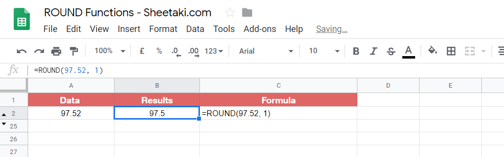
4. Now the fun part! Let’s give our function the value that we want to round up. I’ll be giving a random value of 97.52.

5. You may also give it a number of places, where for now I’ll be putting nothing for it since I just want to round up the 97-part of the value and not the decimal digits. Once you added the places value (if you did for yours) or you followed what I did then make sure to close the brackets ‘()’ as shown below.

6. Finally, just hit your Enter key. You’ll find that if you followed my steps, the value 98 should appear. This is because when your round 97.52 you will get 98 based on the first decimal place.

7. Let’s try another one! This time I’ll be choosing the same number but I’ll be making the places value 1.

8. Following the same steps 1-7, you’ll find that the result would 97.5. Why? Well, it’s because when you round 97.52 the place of 1 will be included with the result number which is 97.5. So 97.52 will be rounded down in this case.

9. Let’s try one last example. This time I’ll be putting -1 as the places.

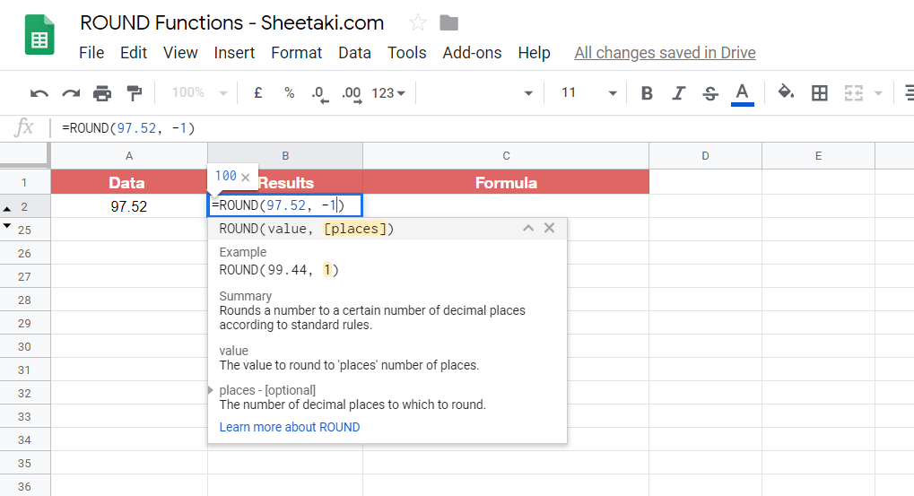
10. You should see that the result will be 100 because the digit rounded will be one place to the left of the decimal point. In this case, it will be 97 which rounds to 100.

That’s pretty much it. You can now use ROUND functions in Google Sheets together with the other numerous Google Sheets formulas to create even more powerful formulas that can make your life much easier. 🙂

Get emails from us about Google Sheets.

Our goal this year is to create lots of rich, bite-sized tutorials for Google Sheets users like you. If you liked this one, you'll love what we are working on! Readers receive ✨ early access ✨ to new content.

Subscribe