How to Use DATEVALUE Function in Google Sheets

The DATEVALUE function in Google Sheets is a simple function used to return the number that represents the date in Google Sheets date-time code. It converts a provided date string to a serial number that represents a date.

So, if we have a list of dates in a variety of formats, and those dates are formatted in Google Sheets as text, we will definitely need this function.

Now, this is the kind of scenario you may come across when you’re importing or downloading data from different sources.

For instance, you may import data from, let’s say your payroll system. Now you have a list of dates that come across as texts. This means they become redundant when you use them in pivot tables and formulas because Google Sheets doesn’t understand them as dates.

So, what this function does is that it ultimately converts the format of a date from text to date. Notice that I said “ultimately” because the value this function returns is still not a date. It’s the number of days since 30-Dec-1899 because that’s the earliest date Google Sheets is capable of.

For example, if you have a text of this date (31-Dec-1899) and you put this text into our function, the result will be 1.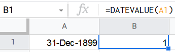

Now, it’s your turn to experiment with some date texts and see what the number the date value returns. If you find any difficulty, the next parts will clear everything up.

Let’s go ahead and look deeper into this interesting function we have in Google Sheets.

The Anatomy of DATEVALUE Function in Google Sheets

Like any other Google Sheets function, the DATEVALUE function has a specific structure that needs to be built in order for it to work.

So, the syntax (the way we write) of the DATEVALUE function is as follows:

=DATEVALUE(date string)

Let’s dissect this thing and understand what each of these terms means:

• = (the equal sign) is just how we tell Google Sheets that we are starting a formula.
• DATEVALUE is the name of the function we are using.
• () These parentheses are used to host the one argument we put in our function.
• (date string) The function’s only argument that takes the date text.

Note that if you don’t input a text value in the DATEVALUE function, you will get an error.

If you want to make sure that your value is of the text format you can set it yourself as follows:

Another thing to be aware of, is that your date text should be in the mm/dd/yyyy format, otherwise you will get an error.

Now for further explanation, let’s go through the DATEVALUE function with an example, and you will master it once you start practicing its application.

A Real Example of Using DATEVALUE Function

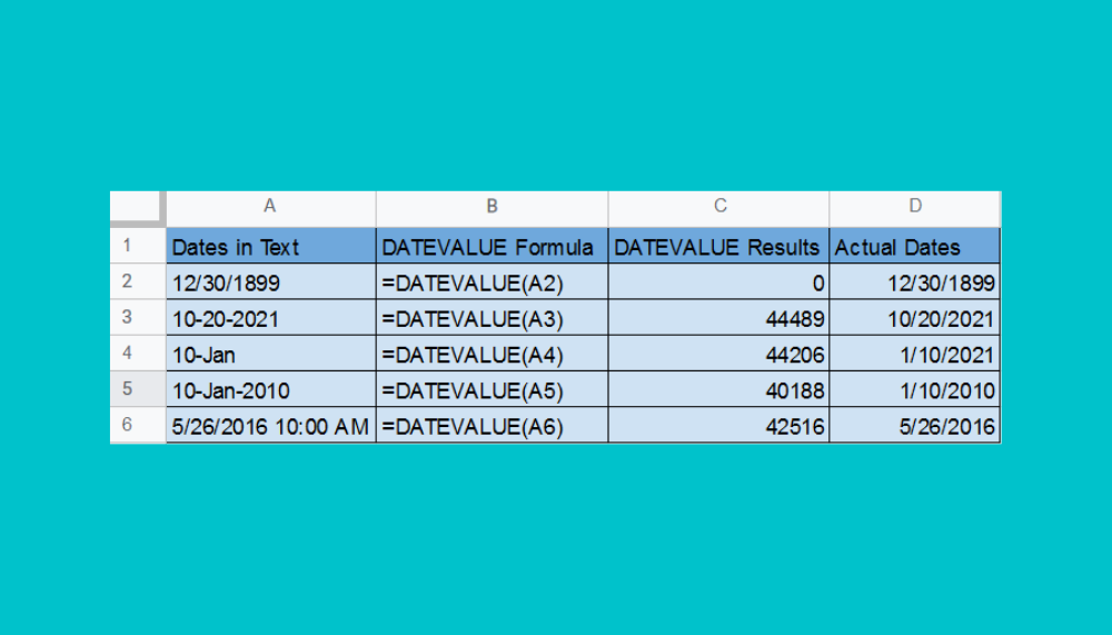
Let’s say we have the following date texts in our Google Sheets:

• 12/30/1899
• 10-20-2021
• 10-Jan
• 10-Jan-2010
• 5/26/2016 10:00 AM

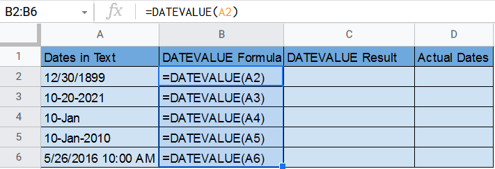
Now, we want to convert these text strings into dates, so we create the following table to illustrate how it’s done.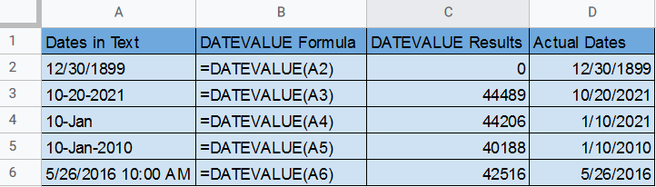

Notice that the values in the ‘Dates in Text’ column are all left aligned which indicates that they are of the text format.

As you can see, we put the DATEVALUE functions in cells B2:B6 to get the corresponding date for each text.

As for the DATEVALUE Results column, here we have the results from each function in Column B.

Finally, in column D we have the DATEVALUE results converted into actual dates with date formatting, therefore they are right aligned.

Now let’s go ahead and create this table from scratch to understand the whole process in the next section.

You may make a copy of the spreadsheet using the link I have attached below.

Make a copy of example spreadsheet

How to Use DATEVALUE Function in Google Sheets

1. First, we write down the column names and the dates we have as follows:
2. Then we click on cell B2, to write our first formula for the DATEVALUE function. So, we type ‘=’ to indicate we are writing a function.
   Then, we type ‘DATE’ and select our function (DATEVALUE) as follows: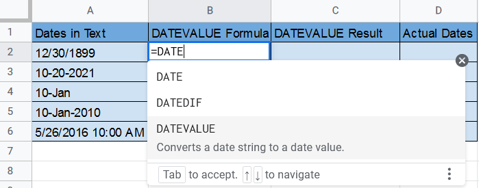
3. We then put in our date text which would be the value in cell A2.
   We see that the result would be 0, since it’s the first ever date in Google Sheets as mentioned before.
4. Now we close the parentheses and press Enter, which will lead to the following pop up.
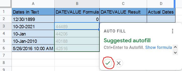
5. We can now click on the tick mark and see what happens.
   You see now the rest of the rows are populated with the results now.
   If you didn’t see that pop up, there’s another way to populate the column, and here it goes:
   You see in the selected cell, that bottom right corner square, when you hover over it, you will see the mouse turned to a ‘+’ sign, double click on it or drag it down and the cells will populate with the right formulas.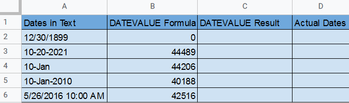
6. Now to view these values as formulas, you click on ‘View’ in the toolbar and select ‘Show formulas.’
7. Then you select the cells B2:B6 and copy them, via pressing ‘Ctrl+C’.
   Now you select cell C2 and paste as values via pressing ‘Ctrl+Shift+v’
   Now do the same thing in cell D2
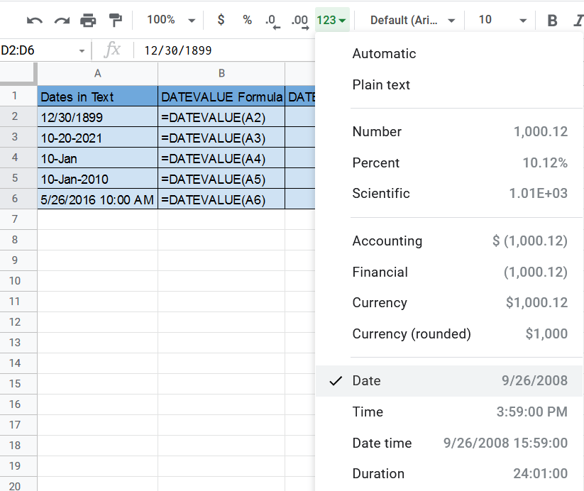
8. Finally, change the format in the D2:D6 cells to the Date format to see the actual dates.Now you have achieved your goal and converted the date texts into actual dates, using the DATEVALUE function.

That’s pretty much it. Congrats! You now mastered the DATEVALUE function in Google Sheets.

There are many more useful Google Sheets functions that you can enjoy learning daily.

Get emails from us about Google Sheets.

Subscribe