The CONCATENATE function in Google Sheets is useful when you need to combine the text of two or more cells together.
Cells passed through the CONCATENATE function are appended as a single string in the same order it was passed.
Table of Contents
The rules for using CONCATENATE in Google Sheets are as follows:
- The function takes two or more cells as an argument then returns a single string made up of the contents of every cell specified.
- The function may also accept ranges (i.e., A2:A5), as well as text strings.
- You may also use the ampersand operator ‘&’ for a more flexible way of writing your arguments.
Let’s look at a quick example.
After conducting a survey with 500 participants, I was able to get various data points from my respondents. They agreed to mention their first, middle, and last name and their age and city of residence.
I later realized that I needed a column for “Full Name” with the format “
Luckily, with the CONCATENATE function I was able to create just the right formula that I could use to automatically populate the “Full Name” column using the data we already have.
My use case is just one way to use the CONCATENATE function in Google Sheets. We can also use the function as an easy way to dynamically produce phrases or sentences with just the right values for each entry.
The function can also be applied to consolidate various inputs into one column. For example, we can use CONCATENATE to combine Street, City, and ZIP Code columns into a single Address column. The CONCATENATE function is simply the best way to merge various different data sources into a single text output.
Let’s learn how to write the CONCATENATE function ourselves in Google Sheets and later use actual values and formulas to see this function in action.
The Anatomy of the CONCATENATE Function
So the syntax (the way we write) the CONCATENATE function is as follows:
=CONCATENATE(String1,String2)
Let’s dissect this thing and understand what each of these terms means:
- ‘=‘ the equal sign is just how we start any function in Google Sheets.
CONCATENATE()is ourCONCATENATEfunction. It will return a single string out of all the arguments passed through it. It should be noted that the order of the arguments are important.- ‘String1’ and ‘String2‘ are the arguments of the
CONCATENATEfunction. These are the strings you want to merge into a single text. It should be noted that there may be two or more such arguments in your formula. These arguments may either be cells or cell ranges (A5,B3:B5) or strings themselves (“Mr.”, “ – “). It should also be noted that the function converts any number to text when they are joined. - Alternatively, the above formula can be rewritten as
=CONCATENATE(String1&String2). In many cases, using an ampersand operator can be a quicker way to build your formulas.
A Real Example of Using CONCATENATE Function
Take a look at the example below to see how CONCATENATE functions are used in Google Sheets.

We have here a list of respondents who have provided their name information. We used the CONCATENATE function to produce the Full Name text seen in Column D.
The formula used is simply:
=CONCATENATE(A2,”, “,B2,” “,LEFT(C2,1),”.”)
Since CONCATENATE simply merges all the text in order, we need to explicitly add spaces between the values to get the result we need.
Alternatively, you can use the ampersand operator for a similar result:
=CONCATENATE(A2&”, “&B2&” “&LEFT(C2,1)&”.”)
You may make a copy of the spreadsheet using the link I have attached below.
The CONCATENATE function also works on ranges.
For instance, the following table can be concatenated like so using just a simple range: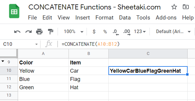
Another thing to note is that Google Sheets has a separate function called CONCAT. The main difference between CONCAT and CONCATENATE is that the former only accepts two strings, and thus is less powerful than our CONCATENATE function.
Great! Let’s begin writing our own CONCATENATE function in Google Sheets.
How to Use CONCATENATE Function in Google Sheets
- Before we type our function, let’s populate our table with some names for us to merge later on.

- To start using
CONCATENATE, we should select any cell to make it the current active cell. For this guide, cell D2 will be where we will input our function’s result. - Next, simply type the equal sign ‘=‘ to begin the function, followed by the name of the function we’ll be using, which is ‘
CONCATENATE‘. - You should find that the auto-suggest box shows you the
CONCATENATEfunction even before fully typing it out. You may press the Tab button on your keyboard to let Google Sheets auto-fill your Formula Bar with “CONCATENATE(“.
As seen below, a tooltip box appears with info on the selected function. We simply hit the arrow on the top-right hand corner of the box to minimize it.

- Let’s type out the arguments we want to combine into one string. In this example, we want to select A2, B2, and C2. Afterwards, simply hit Enter on your keyboard to let the function evaluate.

- We’re almost there! Notice that we still have some formatting left to do. We can add commas and empty spaces into our list of arguments to have a much nicer result.

- We can drag down the
CONCATENATEformula we typed in earlier by placing the cursor at the bottom-right part of the selected cell (it looks like a small blue square) and dragging it down one cell.

Now it looks perfect!
That’s pretty much all you need to know about the CONCATENATE function in Google Sheets. Hopefully, this step-by-step guide has made it easy for you to figure out how to merge your own data.
You can now use the CONCATENATE function in Google Sheets together with the various other Google Sheets formulas available to create more powerful worksheets for your convenience. Do subscribe to our newsletter to be notified of more helpful content like this!