This guide will explain how you can use conditional formatting to highlight every alternate set of N columns in Google Sheets.
Users who want to format their spreadsheets with alternating colors can use conditional formatting rather than setting it up manually.
Conditional formatting makes it easy to highlight certain values or particular cells automatically. In this guide, we’ll use the COLUMN function to determine what column the current cell is in. We’ll use this value to decide whether or not to highlight the cell.
If you need to highlight every other column with a different color, you might find it challenging to perform this manually. The changes are also static and require some effort to reformat.
Using conditional formatting, we can create a dynamic rule that allows you to change how large each set of alternating columns should be.
Now that we know when to use conditional formatting, let’s look at a sample spreadsheet that uses it to highlight alternating sets of columns automatically.
A Real Example of Highlighting Every Alternate Set of N Columns in Google Sheets
Let’s take a look at a real example of the conditional formatting tool being used in a Google Sheets spreadsheet to highlight alternating columns.
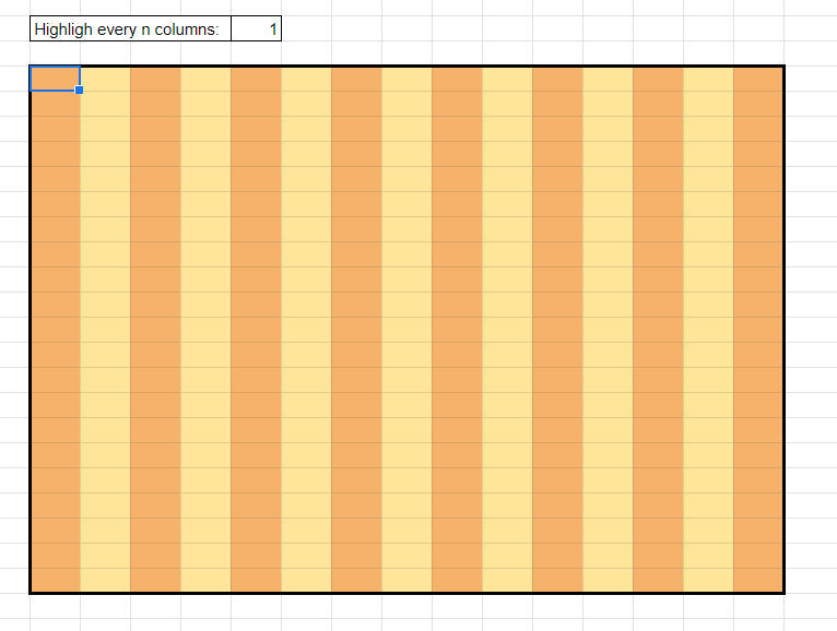
In the example below, the conditional formatting tool has highlighted every other column in the spreadsheet. The size of each set is determined by the value written in cell A1.

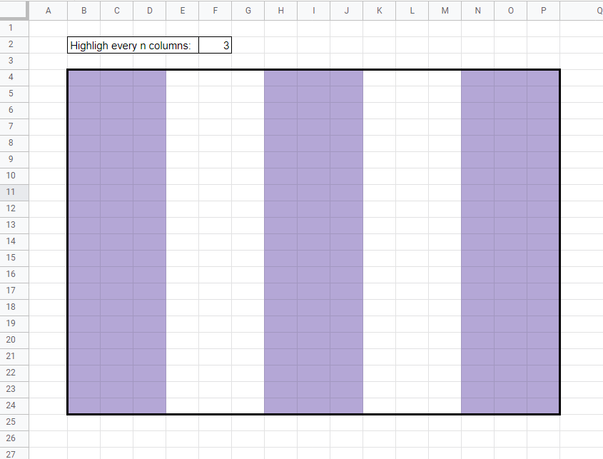
When we change our value in A1 to ‘3’, our conditional formatting rule highlights every other set of three columns in the spreadsheet.

To get this type of pattern, we need to use the following formula in our conditional formatting:
=MOD(COLUMN(A$1)-COLUMN($A$1),$A$1*2)<$A$1
Let’s try to understand what the formula above tries to do. The MOD function finds the remainder after a number is divided by another number. We use the COLUMN function to get the current cell’s column number.
Suppose you want to have an alternating set of two columns. We’re deciding whether to highlight cell G7. We can determine that the cell is six columns away from the first column through the COLUMN function. The MOD function will divide 6 by twice our set size.
This gives us the following formula:
= MOD( 6, 4) < 2
Since MOD(6,4) is equal to 2 and 2 is not less than 2, our formula returns FALSE and does not apply the conditional formatting.
If instead, we choose cell F2, then we’ll get the following formula:
=MOD(6,4) < 2
Since MOD(5,4) is equal to 1 and 1 is less than 2, our formula returns TRUE, and Google Sheets applies the conditional formatting.
In the example below, we’ve added a second conditional formatting rule highlighting the cells between the highlighted columns.

To achieve this, we can use the following custom formula:
=MOD(COLUMN(A$1)-COLUMN($A$1),$A$1*2)>=$A$1
The main difference with this formula is that we substitute the ‘<’ operator with the ‘>=’ operator. This effectively selects the columns we’ve skipped over in the previous formula.
You can make your own copy of the spreadsheet above using the link attached below.
If you’re ready to use conditional formatting to highlight alternate sets of columns in Google Sheets, let’s start writing it ourselves!
How to Highlight Every Alternate Set of N Columns in Google Sheets
This section will guide you through each step needed to highlight every alternate set of N columns in Google Sheets. You’ll learn how to add a custom formula to the conditional formatting tool to help format your spreadsheet.
Follow these steps to learn how to highlight alternate columns using conditional formatting:
- First, select the cells you want to include in your formatting. In this example, we’ll type Ctrl + A to select the entire spreadsheet.

- Next, click on the Conditional formatting tool under the Format menu.

- Under the ‘Format cells if…’ option, select ‘Custom formula is’ in the dropdown box. Paste the MOD formula in the next text box.
You can also select the color you want to use to highlight the chosen columns. Once you’ve entered these settings, click on Done to apply the conditional formatting rules.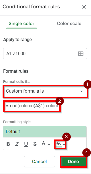
- Since we’ve added a dynamic formula, we must add a number in cell A1. In the example below, specifying a value of 1 highlights every other column.
- You may also select a specific range for conditional formatting. In the example below, we’ve selected the range B4:P24 to be highlighted using our MOD formula.
- If you want two different colors, you may add two conditional formatting rules to the same range.
This step-by-step guide should be all you need to begin highlighting every alternate set of N columns in Google Sheets. We’ve shown how easy it is to use conditional formatting rules to color your spreadsheet with alternating colors automatically.
As this article has shown, we can quickly format a spreadsheet with the conditional formatting tool and custom formulas. With so many other Google Sheets functions available, you can surely find one that suits your use case.
Are you interested in learning more about what Google Sheets can do? Do subscribe to our Google Sheets newsletter to keep up with the latest guides and tutorials from us.