Adding a Custom Formula to a Slicer in Google Sheets

This guide will explain how to start adding custom formulas to a slicer for charts in Google Sheets.

Slicers with custom formulas can help users explore their datasets since they can define what data appears in a chart or pivot table.

Slicer is a Google Sheets tool that allows you to filter tables, charts, and pivot tables. It appears as a floating toolbar that can be placed anywhere on the sheet. 

Each slicer is set to filter a specific range through a particular field. Spreadsheet users can click on the drop-down arrow to apply a filter to that column. 

Slicers can filter by values or by condition. If the user filters by values, they can select or deselect certain values from appearing in the filtered range.

If the user filters by condition, they can filter a column by certain criteria. For example, we can select rows with a blank value or with a value greater than a specific number. Alternatively, they can also provide a custom formula for advanced filtering.

Let’s take a look at a sample use case for using a custom formula in a slicer.

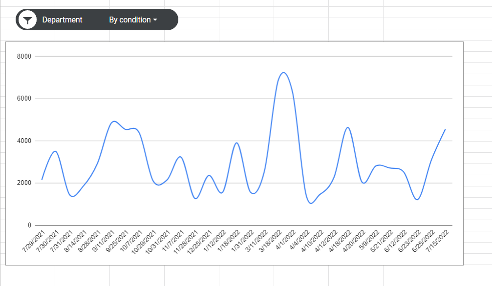
Suppose you have a sales dataset that you’ve visualized using a line chart. You would like to narrow down the dataset to sales from specific departments or teams. 

You can use a slicer to filter the source data of your line chart. If you want to perform an advanced selection, such as selecting all departments that start with ‘C’’, you can use a custom formula as a condition for filtering using a slicer.

This use case is just one way to use the slicer tool in Google Sheets. You can even add multiple slicers to a single dataset to allow the user to filter data using more than one field.

Now that we know when to use a custom formula in a slicer, let’s dive into how it can be used on an actual spreadsheet.

A Real Example of A Custom Formula in a Slicer for a Chart in Google Sheets

Let’s take a look at a real example of a slicer that filters a dataset using a custom formula.

In this example, we will use a dataset of sales data. Each row indicates the sales agent’s last name, their department, the amount in dollars sold, and the entry date.

Using a line chart and a slicer, any user can explore the dataset by changing what the chart shows. In this example, we’ve added a slicer to help select which departments to show in the line chart.

You can make your own copy of the spreadsheet above using the link attached below. 

If you’re ready to try out the slicer tool in Google Sheets, let’s begin setting it up ourselves.

How to Add a Custom Formula in a Slicer for a Chart in Google Sheets

This section will guide you through each step needed for adding custom formulas to a slicer . You’ll learn how we can use the slicer to filter a dataset and modify charts and pivot tables in your spreadsheet.

Follow these steps to add a slicer in Google Sheets with a custom formula.:

1. First, add a new chart to your spreadsheet. In the example below, we’ve added a line chart with sales data in another sheet.
   
   
2. Next, select the ‘Add a slicer’ option that can be found in the Data tab.
   
   
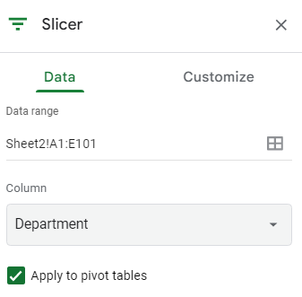
3. A prompt will pop up asking you for the data range that the slicer will filter. In this example, we will use the range Sheet2!A1:E101. Click on the OK button. You may now place the slicer toolbar anywhere in the current sheet.
   
   
4. Select the slicer and look at the panel on the right-hand side. Under the Data tab, select the column you want to slice your data on. In this example, we’ll use the dataset’s Department column.
   
   
5. Click on the Slicer’s dropdown menu to access the filter options.
   
   
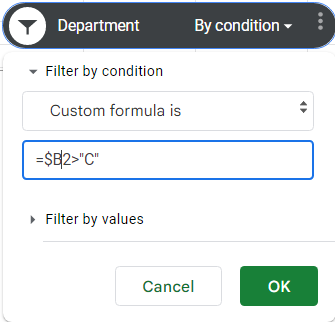
6. Click on the Filter by condition option and select ‘Custom formula is’.
   
   
7. You can now add your own custom formula that will act as criteria for filtering. In this example, we’ll check whether the value in the Department column is greater than the string ‘C’. Once you’ve written your custom formula, click on the OK button.
   
   
8. Finally, your chart should have changed to reflect the newly filtered dataset. Any user with access to the spreadsheet can click on the slicer to change the custom formula when needed.
   
   

This step-by-step guide should be all you need to start adding custom formulas to a slicer in your spreadsheet. Our guide shows how valuable a slicer can be for modifying charts in your spreadsheet.

The Slicer tool is just one example of a feature you can use in Google Sheets to explore your dataset. With so many other Google Sheets functions available, you can indeed find one that suits your use case. 

Are you interested in learning more about what Google Sheets can do? Do subscribe to our Google Sheets newsletter to keep up with the latest guides and tutorials from us.

Get emails from us about Google Sheets.

Our goal this year is to create lots of rich, bite-sized tutorials for Google Sheets users like you. If you liked this one, you'd love what we are working on! Readers receive ✨ early access ✨ to new content.

Subscribe