How to Highlight Multiple Groups and Control Checkboxes in Google Sheets

Highlighting multiple groups using checkboxes in your Google Sheets document makes it easier to read separate groups in your spreadsheet. This is especially useful when you are making a checklist and want to section each checklist off, making it easier for you to keep track.

Google Sheets has a built-in Data Validation and Conditional Formatting features that make data visualization easier. It helps spreadsheets become organized and easily understood – whether the data is numbers or words.

For example, you are shopping for a big party and you are keeping track of each category of goods you need for the occasion. The list could get so long and you can lose yourself in your list. If only there was a way to keep track of everything!

So, how should we go about it?

To accomplish our goal, we have some options we could consider. We can use a combination of ARRAYFORMULA, MATCH and LOOKUP, and even REGEXMATCH functions of Google Sheets.

How to Create Checkboxes in Google Sheets

Before we start highlighting any rows, you should know where to find the checkbox option in Google Sheets.

1. On the menu bar, pick Data, and from the dropdown menu, choose “Data Validation”.

2. In the criteria dropdown menu, go all the way down and pick “Checkbox”.

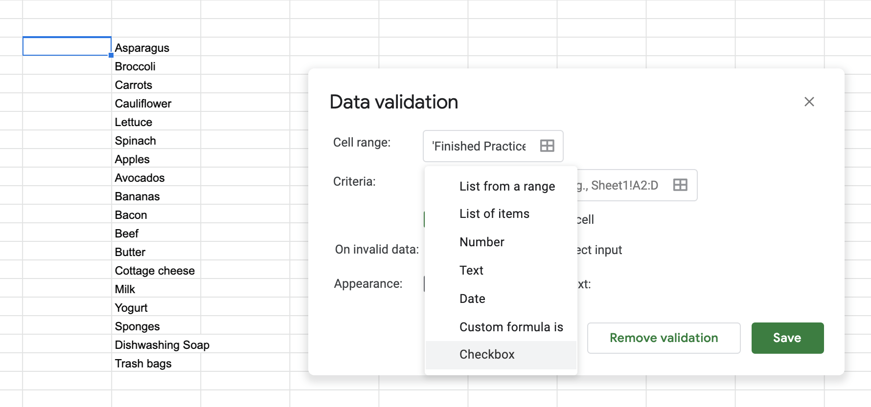
3. That should do it, go ahead and click “Save”.

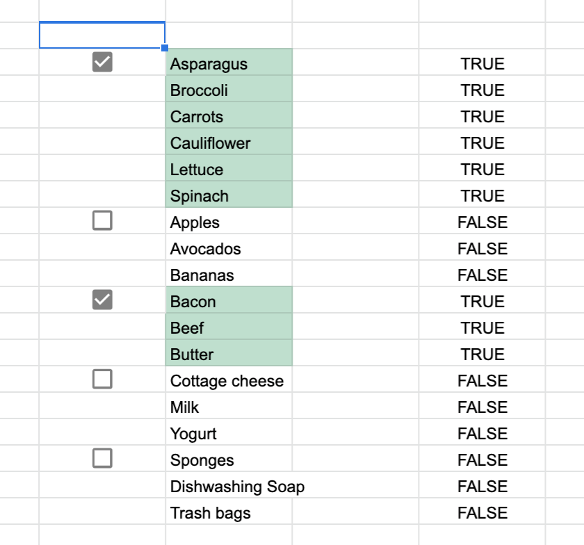
4. There should be a checkbox on the first section of the checklist. Note that when you look at the value of the checkbox, it’s false if unchecked, and true if checked.

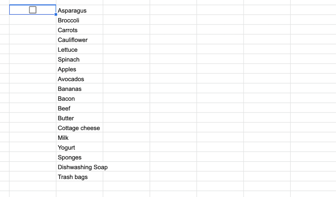
5. Do this for the rest of the list and sections.

How to Highlight Multiple Groups and Control Checkboxes with a Helper Column in Google Sheets

Here is the first option you can choose: put in a “Helper” column.

1. Insert the following formula where you want to start the helper column. Make sure to change the reference arrays as needed.

=ARRAYFORMULA(IF(ROW($B$4:$B<=MATCH(2,1/($C:$C<>""),1),LOOKUP(ROW($B$4:$B),ROW($B$4:$B)/if($B$4:$B<>"",TRUE,FALSE),$B$4:$B),))

2. The ARRAYFORMULA will immediately fill out the rest of the included items.

3. After that, choose Format > Conditional Formatting.

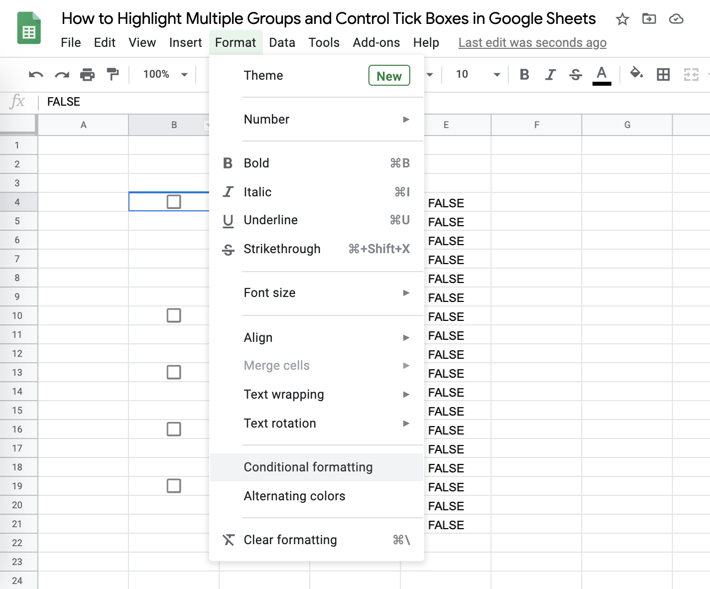
4. Choose the array of your list.

5. Choose Custom Formula from the dropdown menu.

6. Insert the following formula, and click done!
   1.  

=E4=TRUE

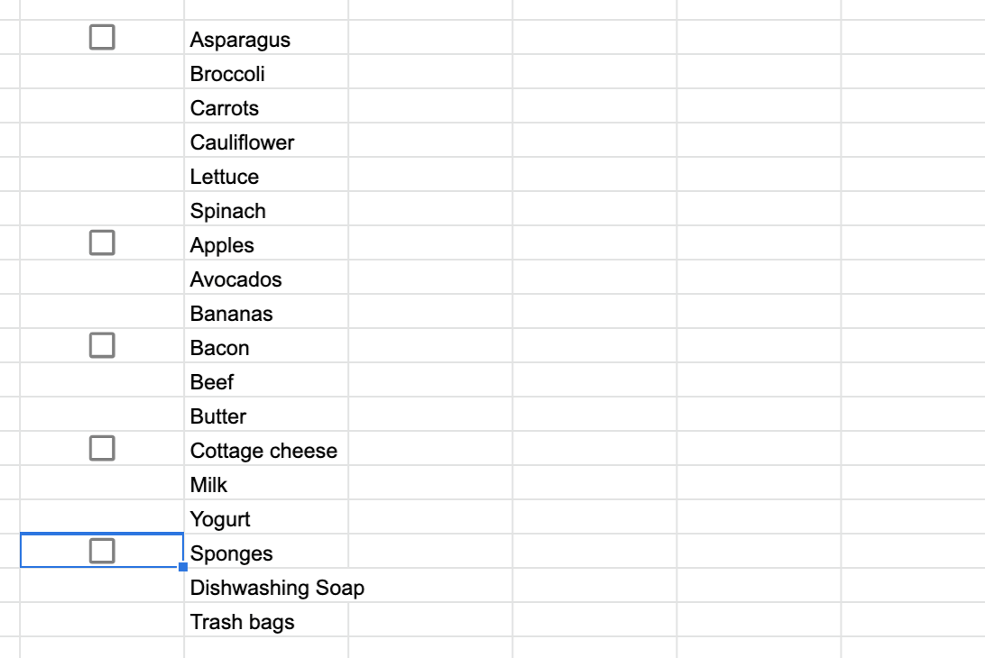
7. Test your highlights now – you will notice checking the box highlights the group that you want!
   

How to Highlight Multiple Groups and Control Checkboxes with the REGEXMATCH Function in Google Sheets

Want to do this without putting in a helper function? There is another option for you, by turning the Helper column into a REGEXMATCH Function in the Conditional Formatting formula.

1. Choose Format > Conditional Formatting.

2. Choose the array of your list, and choose Custom Formula from the dropdown menu.

3. Insert the following formula and click done!

   
   =REGEXMATCH(ROW(B4)&"","^"&textjoin("$|^",true,ArrayFormula(IF(ArrayFormula(IF(ROW($B$4:$B)<=MATCH(2,1/($C:$C<>""),1),LOOKUP(ROW($B$4:$B),ROW($B$4:$B)/IF($B$4:$B<>"",TRUE,FALSE),$B$4:$B),))=TRUE,ROW($B$4:$B),)))&"$")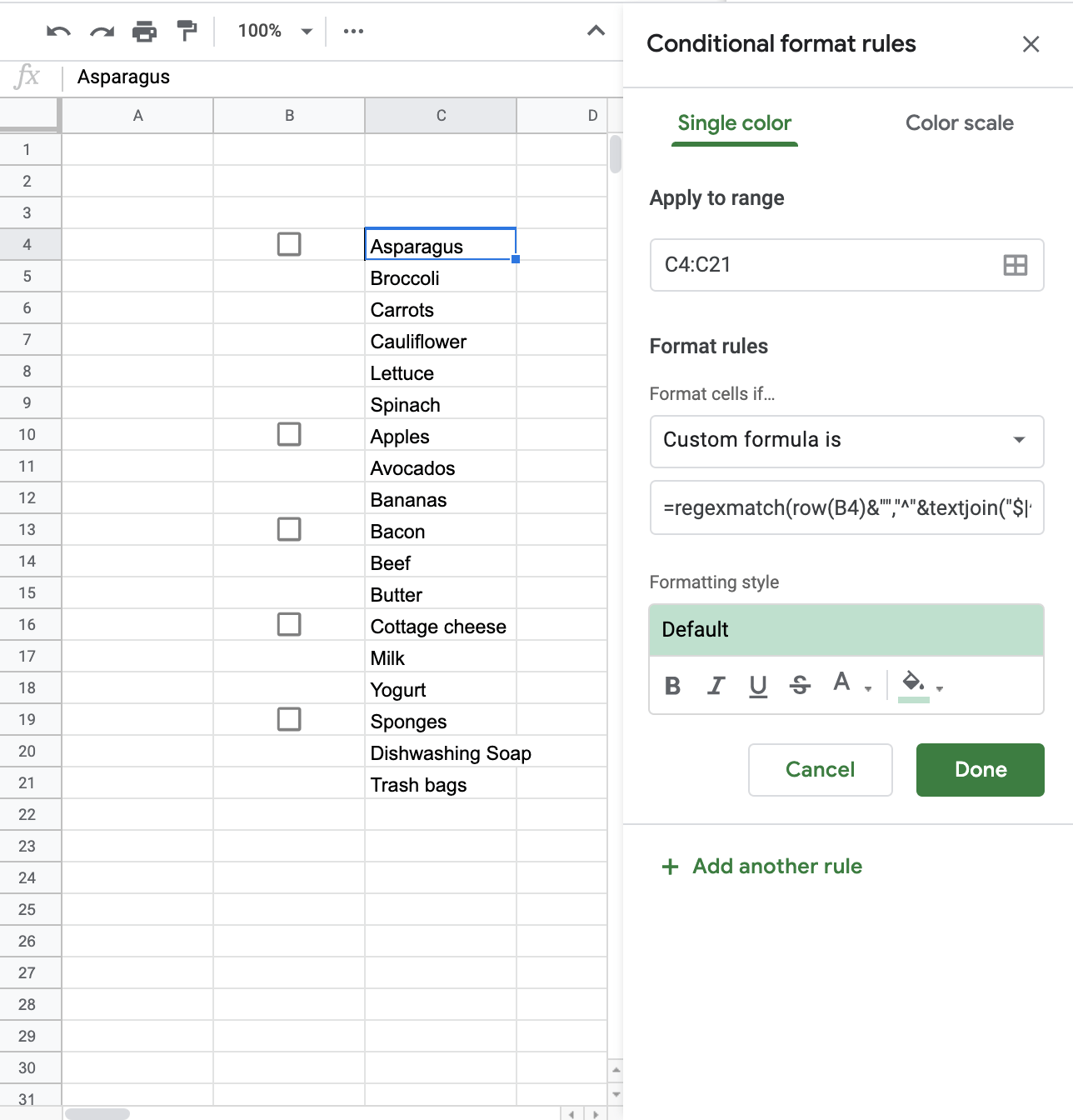

   

4. Test your highlights now – it works just like the previous function!

There you have it! You are now able to highlight multiple groups and control checkboxes in Google Sheets as you wish, without disturbing the integrity of your data.

Now that you have a grasp on how to combine data visualization styles in your spreadsheets, you can combine this with other Google Sheets formulas to make really powerful data documents!

Use the link below to use our spreadsheet sample:

Get emails from us about Google Sheets.

Our goal this year is to create lots of rich, bite-sized tutorials for Google Sheets users like you. If you liked this one, you'll love what we are working on! Readers receive ✨ early access ✨ to new content. There will be no spam and you can unsubscribe at any time.

Subscribe