How to Use the COUPNUM Function in Google Sheets

The COUPNUM function in Google Sheets is used to calculate the number of coupons (interest payments) that will occur between an investment’s settlement date and maturity date.

This financial function is useful because it helps you find out the amount payments that will occur in the time between a given settlement date and maturity date. It is an easy way to calculate it with the given information.

Let’s look at an example.

You have decided to make an investment in bonds. Given a maturity date in 5 years for a quarterly payment schedule, what is the number of coupons or interest payments required between the settlement and maturity date?

How should we go about this problem?

The COUPNUM function takes in all these inputs in order to calculate the number of interest payments.

The Anatomy of the COUPNUM Function in Google Sheets

The syntax of the COUPNUM function is as follows::

=COUPNUM(settlement, maturity, frequency, [day_count_convention])

Let’s check out each part of the function to understand what is going on here:

• = is the equals sign that starts off any function in Google Sheets.
• COUPNUM is the name of our function.
• settlement is the settlement date of the security, which is the date after issuance to the buyer of the delivered security.
• maturityis the end date of a security, which is the date it can be redeemed at face value.
• frequency is the number of interest or coupon payments made annually. This is a digit that corresponds to a certain schedule: 1 for annual, 2 for semiannual, and 4 for quarterly payments.
• day_count_convention is an optional input that is an indicator of which day count method will be in use for the function. This is 0 by default.
  • 0 indicates 30/360 – the US National Association of Securities Dealers (NASD) standard of 30-day months and 360-day years.
  • 1 indicates Actual/Actual – the actual number of days between the specified dates and the actual number of days in the years between the dates. This is used for US Treasury Bonds and Bills and non-financial problems.
  • 2 indicates Actual/360 – the actual number of days between the specified dates and 360-day years.
  • 3 indicates Actual/365 – the actual number of days between the specified dates and 365-day years.
  • 4 indicates 30/360 – the European standard of 30-day months and 360-day years, but with adjustments to end-of-month dates according to European finance standards.

Note that you must input the settlement and maturity dates in a certain format, using DATE,TO_DATE functions to parse the text rather than simply entering the text.

A Real Example of Using the COUPNUM Function

Let’s look at the example below to see how to use COUPNUM function in Google Sheets.

Calculating the Number of Coupons for a Specified Investment in Google Sheets

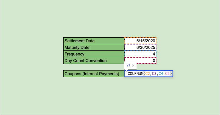
This is a simple problem. We want to find the number of coupons or interest payments between settlement and maturity for a certain investment. The settlement and maturity dates are given below, and we have a quarterly payment frequency. We will use the typical US standard for day count convention.

The function takes four arguments, one of which is optional. So in the equation, it will look like this:

=COUPNUM(C2,C3,C4,C5)

As a result, we get 21 coupons.

This simple problem can be practiced to perfection. Use the link below to get a copy of this problem set:

How to Use the COUPNUM Function in Google Sheets

In this section, we will show you a step-by-step process on how to use the COUPNUM function in Google Sheets.

In this problem, we will calculate the number of interest payments it takes between the settlement and maturity date.

Calculating the Amount of Coupon/Interest Payments in Google Sheets

1. To begin, let’s make sure the information of the dates provided is set with the DATE function, to ensure that no accidental errors will occur from a mistaken input of day, month, and year.

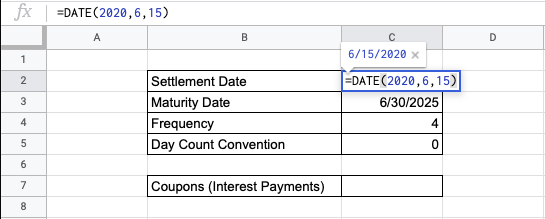
2. Then, click on a cell to make active, which you would like to display the number of coupons. For this guide, the answer will be in Cell C7.

3. Next, type the equal sign ‘=’ to start. Type in “COUPNUM” or “coupnum” – Google Sheets functions are not case sensitive, so you can use either.

4. The auto-suggest box will create a drop-down menu. Select the COUPNUM function by clicking it.

5. After the opening bracket ‘(‘, you will add the settlement date attribute.

6. Next, we enter the maturity date.

7. Next, we enter the frequency of the payments.

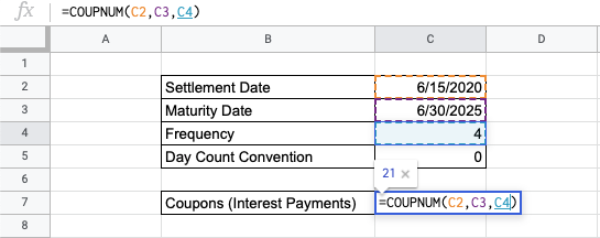
8. Lastly, choose the day count convention. Here we have indicated zero, but you can choose to leave it blank as well. You should be seeing a preview of the final result.

9. Hit Enter and you’re done!

Given a practical problem where you should solve for the correct number of coupons, use the COUPNUM function to find and study the correct input of dates, frequency, and conventions for your important financial decision-making.

And there you have it – you can now use the COUPNUM function in Google Sheets together with the other numerous Google Sheets formulas to create even more effective formulas.

Get emails from us about Google Sheets.

Our goal this year is to create lots of rich, bite-sized tutorials for Google Sheets users like you. If you liked this one, you'll love what we are working on! Readers receive ✨ early access ✨ to new content. There will be no spam and you can unsubscribe at any time.

Subscribe