How to Use AMORLINC Function in Google Sheets

The AMORLINC function in Google Sheets is useful when you need to compute the depreciation of an asset over a certain period.

This function is available for users who follow the French accounting system. It allows the user to calculate the prorated depreciation of an asset purchased in the middle of a given period.

The rules for using the AMORLINC function in Google Sheets are as follows:

• The function requires the user to input the asset’s original purchase cost, salvage value, and other details about the depreciation.
• The function then outputs the depreciation of the asset on the indicated period.

Let’s take a look at a situation where you might want to use this function.

A business owner owns an asset worth $5000. Since this asset loses value over time, he would like to compute how much the asset depreciates over a period of 5 years. He knows that the asset would have a book value of about 750 dollars at the end of its life once it has been fully depreciated. He also knows that the annual depreciation rate is 20% so he wants to sell it before it depreciates to $1000. 

Using the AMORLINC function, he can compute what period he would have to consider selling the asset before the value goes too low.

Let’s learn how to write down the AMORLINC function in Google Sheets and later test out the function ourselves with the values mentioned in our earlier example.

The Anatomy of the AMORLINC Function

So the syntax (the way we write) the DAYS function is as follows:

=AMORLINC(cost, purchase_date, first_period_end, salvage, period, rate,[day_count_convention])

Let’s dissect this thing and understand what each of these terms means:

• = the equal sign is how we start any function in Google Sheets.
• AMORLINC() is our AMORLINC function. It computes the prorated depreciation of an asset on a certain period
• cost refers to the asset’s original purchase cost
• purchase_date refers to the date the asset was purchased
• first_period_end indicates the end date of the first period
• salvage refers to the given asset’s value at the end of its life, when the asset has been fully depreciated
• period is the period we will use for calculating the depreciation. This argument must be a non-negative value. 
• rate refers to the annual depreciation rate to be used in the computation
• day_count_convention is an optional argument that indicates which day count method to use. By default it uses the US(NASD) 30/360 system. This assumes 30-day months and 360-day years.

A Real Example of Using AMORLINC Function

Let’s look into an example of the AMORLINC function being used in a Google Sheet spreadsheet.

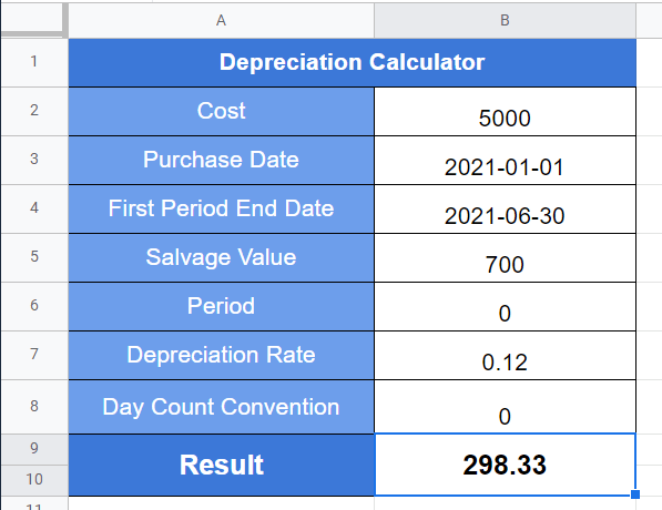
In the table below, we’ve set up our own Depreciation Calculator to help compute the business asset depreciation mentioned earlier.

To get the values in cell B9, we just need to use the following formula:

=AMORLINC(B2,B3,B4,B5,B6,B7,B8)

You can make a copy of the spreadsheet above using the link I have attached below. 

We’ve set up another table to show how the asset depreciates over several periods in the example below. 

Column C uses our AMORLINC formula given the same values as the previous table, with the difference that the period varies based on Column A. We compute the Closing value for that period by subtracting the depreciation from the value of the asset at the start of the period. For example, cell G2 has the formula =B14-C14 and cell B14 carries over the value of D13 in the row above. This table indicates that the business owner should try to sell his asset by the sixth period if he would like to claim a value over 1000 dollars.

If you’re ready to try out the AMORLINC function in Google Sheets, let’s begin writing our own Depreciation calculator ourselves!

How to Use AMORLINC Function in Google Sheets

1. To start our depreciation calculator, we’ll need to input some values into our spreadsheet. The table below has all the necessary arguments we need to compute for the depreciation.
   
   For this example, we’re computing the depreciation after the first period (indicated with a 0) of an asset worth $5000 with a depreciation rate of 12%.
   
   

1. To use the AMORLINC function, first select the cell we will first put our function’s output. In this example, we’ll place our result in cell B9
2. Next, we just need to type the equal sign ‘=‘ to begin the function, followed by ‘AMORLINC(‘. 
3. As seen below, a tooltip box appears with info on the AMORLINC function. We can click on the arrow on the top-right-hand corner of the box to minimize it if necessary.
   
    
4. The next step would be to reference all the needed arguments into your function. Thanks to our table, we simply need to reference each cell in order.
   Afterwards, simply hit Enter on your keyboard to let the function evaluate.
   
    
5. Once the formula has been evaluated, we now know that the asset has depreciated $298.33 in the first period.
   
   

After following all these steps, you’ve successfully learned how to use the AMORLINC function in Google Sheets. This step-by-step guide shows how easy it is to compute depreciation in Google Sheets!

You can use the AMORLINC function in Google Sheets together with the various other Google Sheets formulas available to create powerful worksheets for business or personal use.

Stay notified of new Google Sheets guides like this by subscribing to our newsletter! 

Get emails from us about Google Sheets.

Our goal this year is to create lots of rich, bite-sized tutorials for Google Sheets users like you. If you liked this one, you'll love what we are working on! Readers receive ✨ early access ✨ to new content.

Subscribe