Highlighting a set of alternate rows in your Google Sheets document makes it much easier to handle your spreadsheet, especially if it has become particularly massive. It becomes increasingly easy to get lost in the rows and columns of data if you’re not careful, so it’s best to use a visual guide while you use your spreadsheet. In this article, we will show you how to highlight a set of alternate rows in Google Sheets.
Table of Contents
Google Sheets has the built-in Conditional Formatting feature that is very useful for ease of data visualization. It makes your spreadsheet not only efficiently organized, but visually appealing as well.
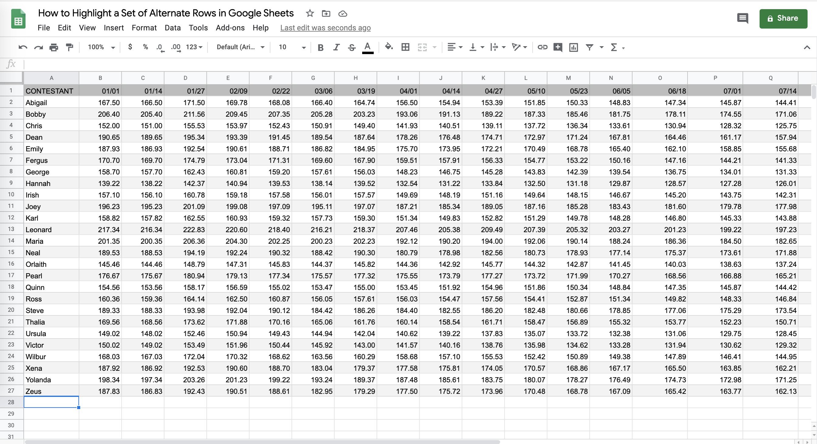
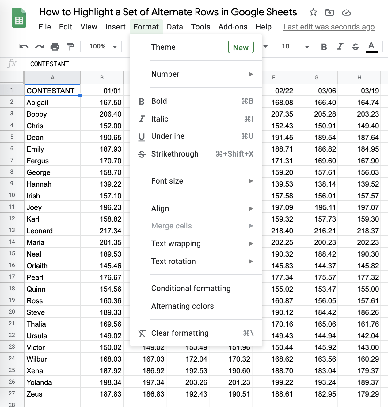
For example, you are hosting a fitness challenge and are keeping track of the contestant check-ins. After a while the list gets so long and the numbers can be so similar – it’s easy to lose track!
So, how should we proceed?
To accomplish our goal, we will use a combination of the ISODD, ISEVEN and ROW functions with the Conditional Formatting feature of Google Sheets.
How to Use Conditional Formatting to Highlight a Set of Alternate Rows in Google Sheets
Here, you can check out conditional formatting automatic solution to highlighting a set of alternate rows in Google Sheets.
- Choose Format from the menu bar. Find and click the option of “Alternating colors“.

- From there, Google Sheets will automatically find your data spread and give you options for alternating row choices, including the header.
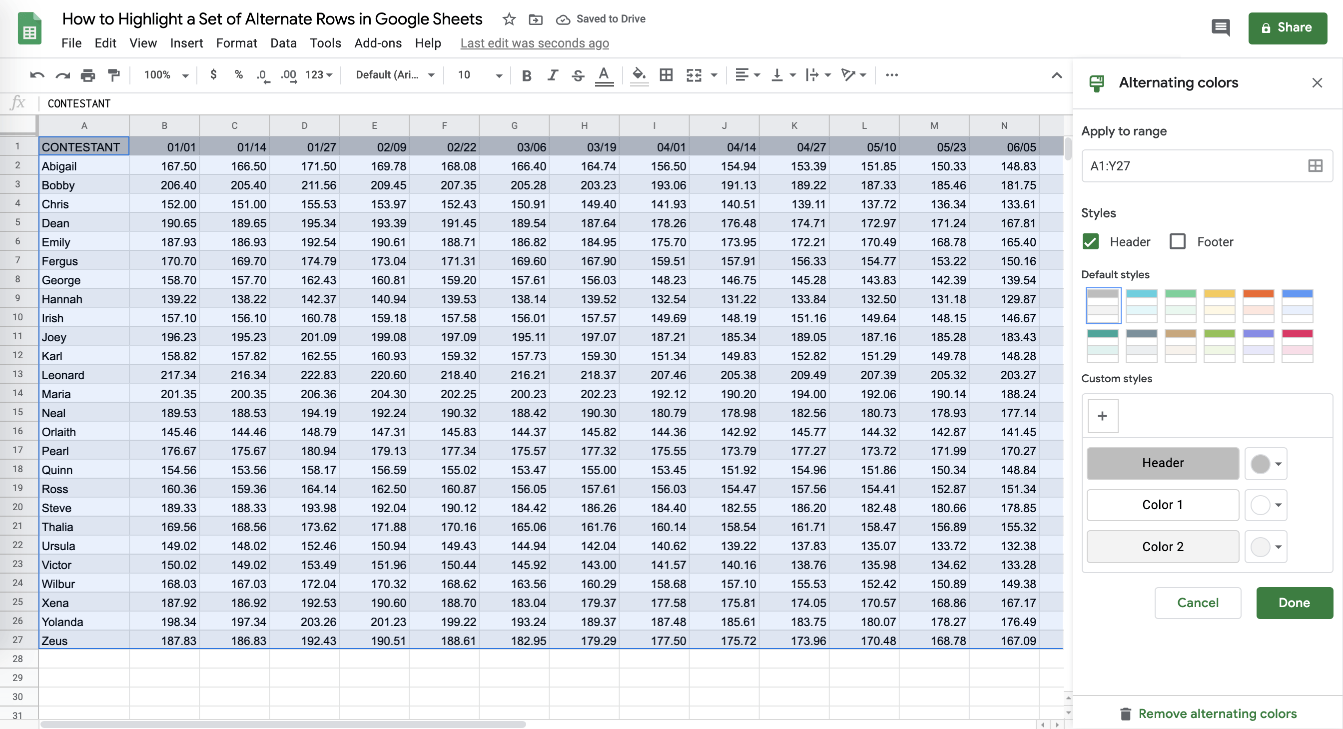
- Customize how you see fit, and you’re done!
This simple problem can be practiced. Use the link below to use our spreadsheet sample:
The Anatomy of the ISODD and ISEVEN Functions in Google Sheets
The syntax (the way we write) the ISODD function is simple:
=ISODD(value)
And the ISEVEN function is similar:
=ISEVEN(value)
Let’s break both of these functions down to understand each term:
=the equal sign is how we begin any function in Google Sheets.ISODDorISEVENis our function. This is what we will use to determine whether a value, whether inputted as a number or as a cell address, is even or odd.valueis the only attribute of this function and
ISODD and ISEVEN are Boolean functions. ISODD will return TRUE if the value is an odd integer or a reference to a cell containing an odd integer, and returns FALSE otherwise. ISEVEN acts the same with even integers.
The syntax of the ROW function is simple:
=ROW([cell_reference])
=the equal sign is how we begin any function in Google Sheets.ROWis our function.cell_referenceis the cell whose row number will be returned. This entry is optional, and if you leave theROWfunction cell reference blank, the cell in which the formula is inputted will be the default.
We will combine these functions together to highlight a set of alternate rows in Google Sheets.
How to Highlight a Set of Alternate Rows in Google Sheets
Aside from the automated method in Google Sheets, here is another function that highlights odd and even rows in Google Sheets.
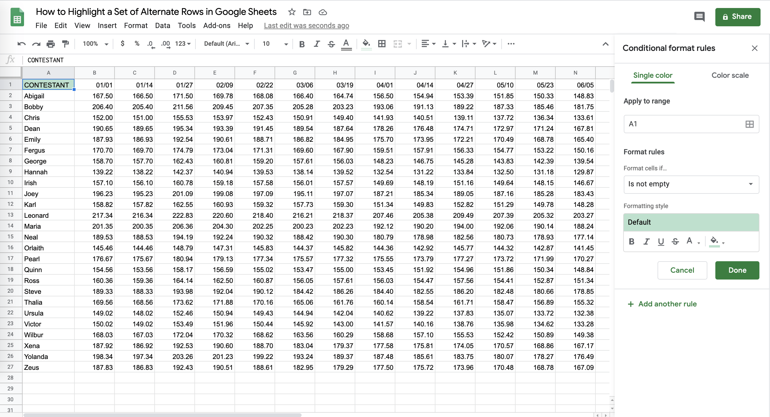
- Choose the Conditional formatting option from the Format option on the menu bar.
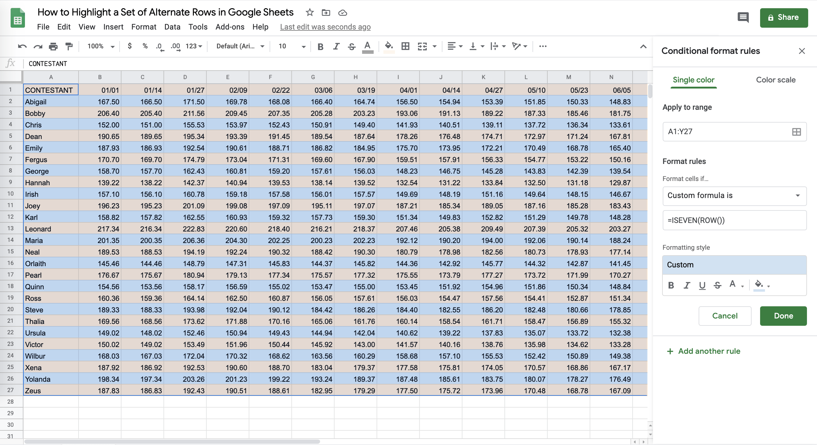
- The conditional format rules box will pop up on the right side of the screen.
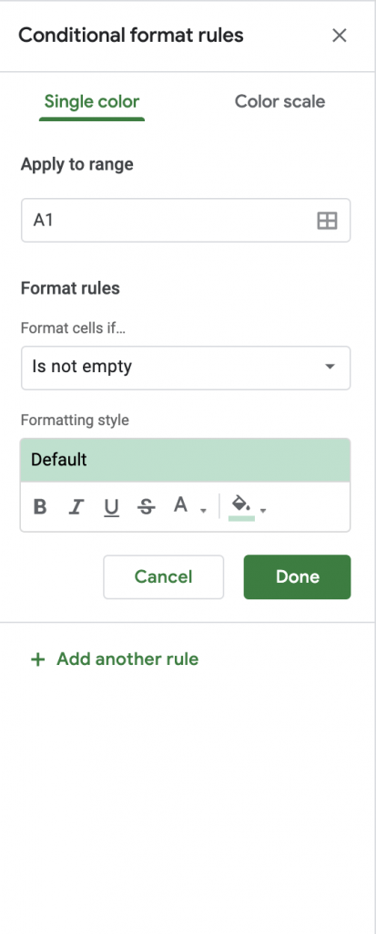
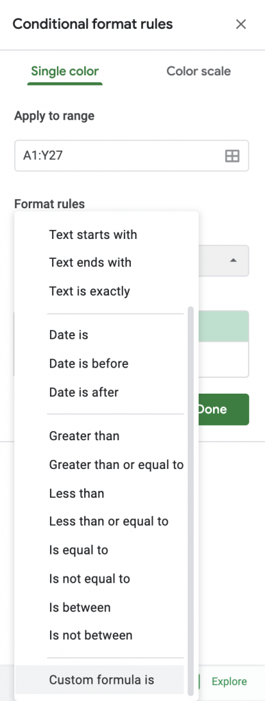
- Select the range you want to apply the alternating rows to take effect.

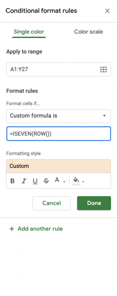
- After you have chosen the range, from the dropdown of “Format rules,” choose “Custom formula is” all the way at the bottom.
- Insert the following formula:
=ISODD(ROW())in the box.
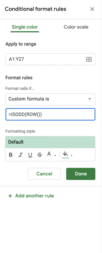
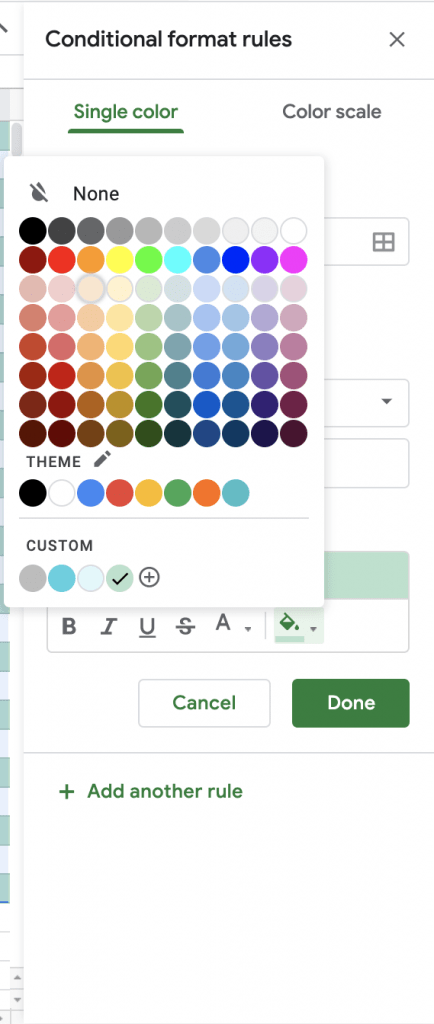
- Customize the formatting style as you wish.
- One set of rows will be properly colored.

- Next, choose the “Add another rule” and add another custom formula, this time with
=ISEVEN(ROW())and customize as you like.
- There you have it! 🙌
How to Highlight Every Nth Row in Google Sheets
Maybe you’re interested to highlight every 3rd or 4th or 5th row in your table, what have you. There is also another way to use Conditional Formatting to return your desired table.
- Choose conditional formatting to add a new rule.
- Add this formula:
=MOD(ROW(),3)=0. Replace N with the number you want. In this example, it’s every 3rd row. Don’t forget to add “=0” at the end, otherwise the effect will be to color every row except the 3rd one!

- Customize as you see fit, and admire your work!

There you have it! You are now able to highlight a set of alternate rows in Google Sheets as you wish, without disturbing the integrity of your data. Now that you have a grasp on how to combine data visualization styles in your spreadsheets, you can combine this with other Google Sheets formulas to make really powerful data documents!