

This guide will explain how you can use Google Sheets functions and conditional formatting to highlight adjacent duplicates in your spreadsheet.
You’ll learn how you can use a formula to determine whether a cell’s value is a duplicate of its adjacent cell. We can later apply this formula as a rule for conditional formatting.
A cell is an adjacent duplicate if it contains a value that appears in the cell immediately preceding it. The location of the preceding cell depends on whether we’re checking duplicates by row or column.
When performing a row-wise check, the duplicate is any cell with a value that is equal to the cell directly to the left of it. In a column-wise check, we’ll check if a cell contains the same value as the cell directly above the current cell.
Let’s take a look at a basic scenario where we can use conditional formatting to highlight adjacent duplicates.
Suppose you have a random list of numbers in Google Sheets. You’ll use these numbers to help you decide what to cook for dinner. For example, a ‘1’ indicates that you must cook a chicken dish.
Since you want to avoid using the same type of meat twice in a row, you want to know if there are any days from the random list that have adjacent duplicate numbers.
We can highlight adjacent duplicates using conditional formatting. We’ll use a formula that determines whether the current cell has the same value as the previous cell.
Now that we know when to highlight adjacent duplicates in Google Sheets, let’s look at several sample tables with the right conditional formatting rules.
A Real Example of Highlighting Adjacent Duplicates in Google Sheets
Let’s take a look at a sample spreadsheet that uses conditional formatting to highlight adjacent duplicates in Google Sheets.
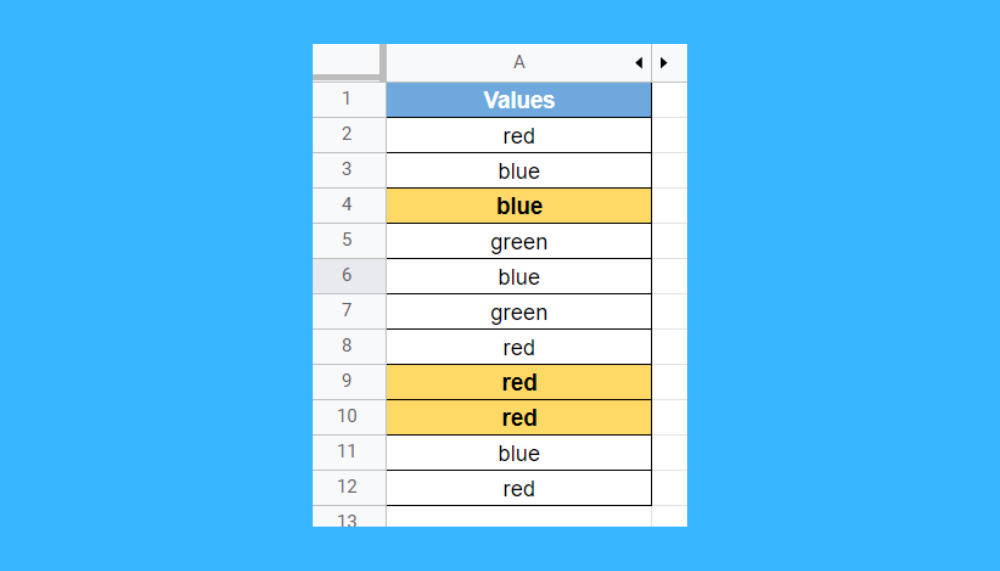
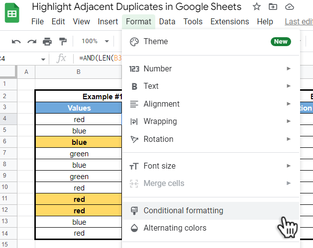
In the example below, we have three highlighted cells in our dataset. Since we’re performing a column-wise check, cell A4 is highlighted because it has the same value as the cell directly preceding it. Similarly, cells A9:A10 are highlighted because they share the same value as cell A8.
To highlight these values, we just need to use the following formula:
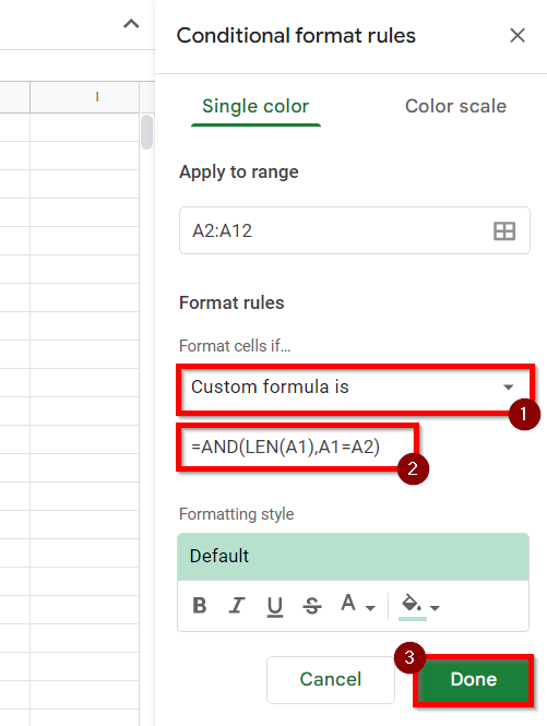
=AND(LEN(B3),B3=B4)
Let’s try to understand how this formula works. The AND function returns TRUE only if both arguments are TRUE. The first argument checks if the previous cell is empty. The second argument checks if the current cell’s value is equal to the previous cell. If both these arguments are TRUE, then the current cell is highlighted.
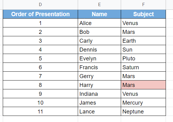
In this second example, we use the adjacent duplicates formula to check if two consecutive students are presenting a report on the same subject. In our example, Harry’s topic is highlighted because he shares the same subject with the previous presenter.
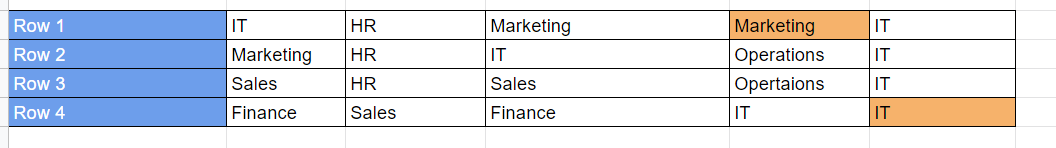
For this third example, we’re using a row-wise check to ensure that people from the same team are seated apart from each other.
To properly highlight adjacent duplicates, we use the following formula:
=AND(LEN(B2),B2=C2)
You can make your own copy of the spreadsheet above using the link attached below.
If you want to start highlighting adjacent duplicates in Google Sheets, proceed to the next section to read our step-by-step guide!
How to Highlight Adjacent Duplicates in Google Sheets
This section will guide you through each step needed to start highlighting adjacent duplicates in Google Sheets. You’ll learn how to add a custom formula to define a conditional formatting rule.
Follow these steps to start highlighting adjacent duplicates :
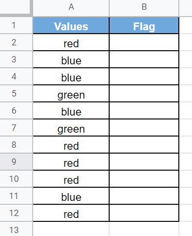
- First, we can add a new column that will determine whether a given value is a duplicate of an adjacent value.
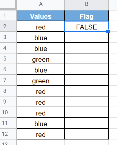
- Next, we’ll add the formula
=AND(LEN(B1),B1=B2)to the first empty row of our new column. Hit the Enter key to evaluate the function.
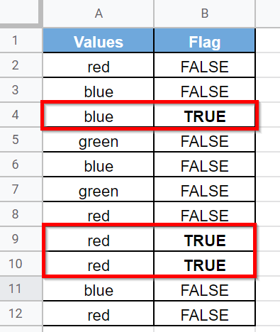
- Use the Fill Handle tool to add the formula to the rest of the column. In the example below, several cells are flagged as duplicates.
Since we want to highlight adjacent duplicates, we will have to use conditional formatting.
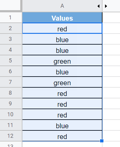
- First, select the range that you want to apply conditional formatting to. In this example, we’ll select the range A2:A12.
- In the Format menu, click on the Conditional formatting option to apply conditional formatting to the current selection.
- In the Conditional format rules panel on the right-hand side of the screen, enter the formula used earlier as a custom formula. You may also specify how you want to format your cell if the formula returns TRUE. Click on Done to apply the custom rule to the selected range.
- After applying conditional formatting, Google Sheets should now highlight cells with adjacent duplicates. In the example below, cells with duplicates are highlighted with a yellow background.
This step-by-step guide should be all you need to start highlighting adjacent duplicates in your spreadsheet. We’ve shown you how to use a Google Sheets formula to define a rule for conditional formatting.
This guide shows just one way you can use conditional formatting in Google Sheets. Rules for conditional formatting can use any type of custom formula. With so many other Google Sheets functions available, you can surely find one that suits your use case.
Are you interested in learning more about what Google Sheets can do? Subscribe to our newsletter to find out about the latest Google Sheets guides and tutorials from us.


