How to Compare Two Sheets in Google Sheets

Learning how to compare two sheets in Google Sheets is useful to identify matches and differences between two different Google Sheets.  

As a frequent Google Sheet user, you may be tasked to scan through two sheets to spot and point out the differences in data. Manually examining takes up too much time and strains our eyes. 👀 

Hence, we are here to demonstrate several effective ways to compare two Google Sheets, namely:

1. Using the Equal Sign
2. Using the IF Function
3. Add-ons Tool

 

 

Using the Equal Sign to Compare Two Sheets

We can easily use the equal sign = to compare values between two columns or two sheets in Google Sheets.

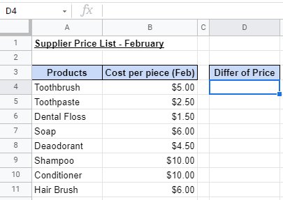
Let’s say you are a toiletry retailer that sells different toiletries ranging from toothbrushes to deodorants. Every month, you would be receiving a price list from your supplier for you to restock your inventories.

You have received the price list for February and would like to compare the prices listed against the previous month. As there are many products on the price list, it is time-consuming to compare them manually. 

Not to worry! We are here to show you how you can compare the price list more efficiently.

Do take note that the above scenario would be adapted for all examples used within the tutorial. 

 

Example 1:

 

As you can see, these are two different sets of price lists extracted from two sheets. 

1. Select the range that you would like to compare from the “Jan” tab. In this example, it would be B3:B11. 

 

2. Then, copy the selected range and paste it into the “Feb” tab. Your sheet would now contain two columns of “Cost per piece”. 

 

3. To avoid confusion, rename the respective headers. 

 

4. Now, let’s input the formula. First, click on the cell that you want to write down your formula. In this example, it will be F4.

 

5. Begin your formula with an equal sign =, then select the value that you want to compare from Jan, which is D4.

 

6. Then insert another equal sign =, followed by the value that you want to compare from February, B4.

 

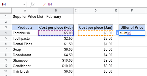
7. After you press Enter, your return value should show “TRUE” or “FALSE”.

 

8. As shown below, rows 8, 9, and 10 have a return value of “FALSE” as there was a price increase. 

 

Example 2:

Instead of copying the values from one tab to another, here is a more direct way. 

1. Select the cell you would like to input the formula in. In our case, it would be D4.

 

2. Similar to Example 1, begin your formula with an equal sign=. Then, select the value that you want to compare from Feb, which is B4. 

 

3. Next, insert another equal sign= and select the value to compare against in the “Jan” tab, which is Jan!B4.

 

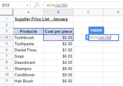
4. Once you press Enter, the same return values would appear. 

 

Using the IF Function to Compare Two Sheets

 The IF function is a very versatile function that can be applied to different scenarios. The function is used to evaluate whether the data you selected meets certain criteria in a logical test, where the result is always “TRUE” or “FALSE”. 

Here is the syntax (the way we write) of IF function:

=IF(logical_expression, value_if_true, value_if_false)

You can visit our tutorial on the IF function before proceeding to appreciate the formula! 

Compared to using the equal sign to compare values, the IF function can tailor the return values if it’s “TRUE” or “FALSE”. You would have a better understanding of how this works after we go through some examples. 

 

Example 1:

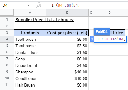
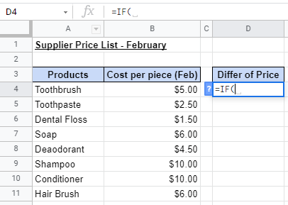
1. Select the cell you would like to input the function in. In our case, it would be D4.

 

2. Begin your function with an equal sign=, then followed by the name of the function, IF, then an open parenthesis(.

 

3. Similar to using the equal sign =, we will input the price we would like to compare against the price in the “Jan” tab. This would be our logical_expression. The formula would look like this:

 

4. Now we would need to add the value_if_true and value_if_false. In this example, we would use “Match” and “Differ” as our respective values. Remember to add a comma , between each attribute! 

 

5. Similar to using the equal sign =, rows 8, 9, and 10 have a return value of “Differ” as the price in January and February do not match. 

 

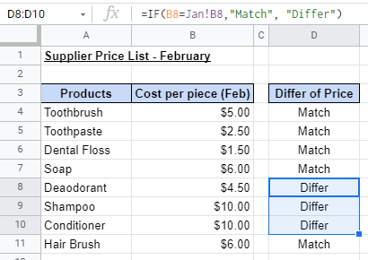
As mentioned earlier, we can alter the return value for both “TRUE” and “FALSE” to any customized value. In this example, it is “Match” and “Differ”.

However, if you would like to visualize how the price differs from January to February, there is another way to do so. 🧐

 

Example 2:

In this example, we would be able to use the IF function to show only those cells that differ in price. 

The formula will pull records from both tabs and separate them with a character of your choice entered into the formula. 

Let’s start!

1. Select the cell you would like to input the function in. In our case, it would be D4. Begin your function with an equal sign =, then followed by the name of the function, IF, then an open parenthesis(.

 

2. Just like the previous example, we will input the price we would like to compare against the price in the “Jan” tab. This would be our logical_expression. The formula would look like this:

 

3. In this example, if the value is “TRUE”, we would like the return value to be blank. If the value is “FALSE”, we would like the return value to show the prices from the “Jan” and “Feb” tabs. 

 

4. For value_if_true, we will input double quotations "" and leave a spacing in between. This will cause the return value to be blank if the value is “TRUE”.   

 

5. For value_if_false, we will input the price in February, which is B4. To add a character in the two prices, input the double quotations "" and insert the desired character. In our case, it would be a vertical bar |. We would then end the formula with the price in January, which is Jan!B4. 

 

Don’t miss out on the ampersand signs &. It is used to connect or join the inputs together to form a string!

 

6. Let’s close the formula with a close parenthesis ). Your final input should look like this:

Final formula: 

=IF(B8=Jan!B8,” “, B8&“|”&Jan!B8)

 

7. To make the return value look less cluttered, we can add spacing in between. 

Final formula: 

=IF(B8=Jan!B8,” “, B8&” | “&Jan!B8)

 

With this formula, you can see the difference in price without referring to the other sheet. This also creates a tidier compared to the previous examples as it shows only the relevant information. 

 

Example 3:

This example demonstrates how we can insert the VLOOKUP function into the IF function for a different situation.

As shown in the images above, the sequence of the products in the “Jan” and “Feb” tab is different. This is where the VLOOKUP function comes into play. 

The VLOOKUP function would allow us to pull out data from a table. In our scenario, the function would help us match the correct product price from January to the selected product price in February. 

Here is the syntax (the way we write) of the VLOOKUP function:

=VLOOKUP(search_key, range, index, [is_sorted])

If you are not familiar with the VLOOKUP function, don’t be shy, and head over to our tutorial on the VLOOKUP function. The tutorial will help with your understanding of the function before we proceed with some examples. 

Let’s go through this step-by-step!

 

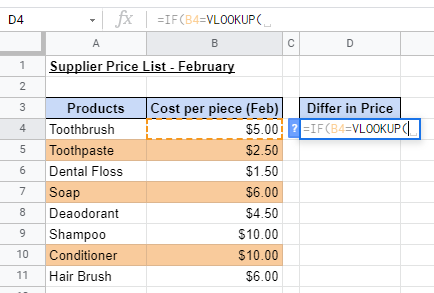
1. Select the cell you would like to input the function in. In our case, it would be D4. Begin your function with an equal sign =, then followed by the name of the function, IF, then an open parenthesis (.

 

2. We will then input the price we would like to compare against the price in the “Jan” tab. This would be our logical_expression. However, instead of inserting the equal sign and the price of the product from the “Jan” tab directly, we would insert the VLOOKUP formula. 

 

3. The first attribute is search_key. In our example, it would be A4. 

 

4. Then, we will insert the range we would like to search from the “Jan” tab, which would be Jan!A4:B11. Don’t forget to add the dollar sign $ to lock the range. 

 

5. Next, we insert “2” as our index attribute. This signifies which value to be returned. In our case, it’s “2” as the price of the product is in column 2. We will end the formula for the VLOOKUP function by inputting “false” to signify that our database is not sorted. 

 

6. Once we are done with the VLOOKUP function, we will then input the values to return in the IF function. In our case, it would be “Match” and “Differ”.

 

7. The final result would be the same as the previous examples:

 

If you are wondering, is there a way to compare two sheets in Google Sheets using just a built-in tool? The answer is yes! You can do so by using the ‘Add-ons‘ tool!

 

 

Using the Add-ons Tool to Compare Two Sheets

The “Add-ons” tool is an advanced tool where you can install different add-ons from the Sheets Add-ons store. 

To compare two sheets in Google Sheets using the ‘Add-ons‘ tool, follow the steps below! 🤗

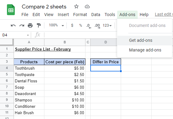
1. Select the ‘Add-ons‘ tool, then select ‘Get add-ons‘. 

 

2. A pop-up for the Google Workplace Market would appear. We would then input ‘Remove Duplicates‘ into the search bar. A variety of add-ons would appear. We would then select the first icon by Ablebits. 

 

3. After selecting the add-on, an overview of the add-on would appear. We will then select Install. 

 

4. A message box would appear to prompt you to allow permission for the add-on to proceed with the installation. We would press Continue.

 

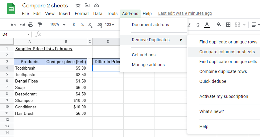
5. Once the installation is complete, the ‘Remove Duplicates‘ tool would appear. We would select the tool, and select ‘Compare columns or sheets‘. 

 

6. For the main sheet, we would select ‘Feb‘ and table A4:B11. This is where the returning value would be recorded. 

 

7.  After pressing Next, we would then need to select the data to compare with, which is the second sheet. In this example, the second sheet would be ‘Jan‘ and the second range of data being A4:B11.

 

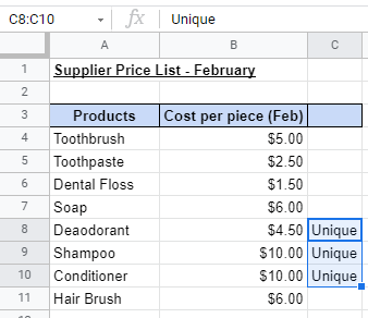
8. To see the products with price changes from January to February, we would select ‘Unique Values‘.  

 

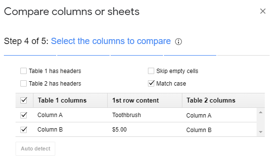
9. In Step 4, we would need to specify how we would like to compare the data between sheets.  As we did not include the headers within the range selected, let’s untick the ‘Table has headers‘ options. 

 

10. Finally, in the last step, we would select the option to ‘Add a status column‘.  Remember to press Finish to complete the process! 

 

11. Our final input would look like this:

 

You may make a copy of the spreadsheet using the link attached below and try it for yourself:

There you go! We have shown numerous ways to compare data from two sheets varying from simple to more complex ways. 

Believe it or not, there are many more methods to compare two sheets in Google Sheets. Don’t hesitate to subscribe to our newsletter to find out how in the future!